Training a FESTIM surrogate model#
Objectives
Use AutoEmulate to build an emulator/surrogate model of a FESTIM problem
Save the emulator to a file for reuse
Build a simulator#
We start by building a simulator (high fidelity) using FESTIM. Here for demonstration purposes we make a simple unit square example with two volume subdomains with different diffusivities. The physical process models hydrogen transport (diffusion) across the two subdomains, driven by the respective source terms. Hydrogen diffuses from the areas of higher concentration towards the boundaries. We are modeling this at a constant temperature.
The model is parametric and takes the volumetric source terms in each subdomains as inputs and returns the total species inventories in both subdomains.
The concentration of species on the boundary of the domain is set to zero.
See also
Check out the AutoEmulate tutorials for more information.
Note
This specific example isn’t particularly expensive to run. Building a surrogate of a FESTIM model is especially useful for large and computationally expensive models, such as 3D simulations with complex geometries, coupled multiphysics (e.g., heat transfer and trapping), or parameter sweeps where a single full-fidelity FESTIM run could take minutes to hours.
import festim as F

from dolfinx.mesh import create_unit_square
from mpi4py import MPI


def make_model(source_bottom: float, source_top: float) -> F.HydrogenTransportProblem:
    fenics_mesh = create_unit_square(MPI.COMM_WORLD, 20, 20)

    festim_mesh = F.Mesh(fenics_mesh)

    material_top = F.Material(D_0=0.2, E_D=0)
    material_bot = F.Material(D_0=0.1, E_D=0)

    top_volume = F.VolumeSubdomain(
        id=1, material=material_top, locator=lambda x: x[1] >= 0.5
    )
    bottom_volume = F.VolumeSubdomain(
        id=2, material=material_bot, locator=lambda x: x[1] <= 0.5
    )

    boundary = F.SurfaceSubdomain(id=1)

    my_model = F.HydrogenTransportProblem()
    my_model.mesh = festim_mesh
    my_model.subdomains = [boundary, top_volume, bottom_volume]

    H = F.Species("H")
    my_model.species = [H]

    my_model.temperature = 400

    my_model.boundary_conditions = [
        F.FixedConcentrationBC(subdomain=boundary, value=0.0, species=H),
    ]

    my_model.sources = [
        F.ParticleSource(species=H, volume=bottom_volume, value=source_bottom),
        F.ParticleSource(species=H, volume=top_volume, value=source_top),
    ]

    my_model.settings = F.Settings(atol=1e-10, rtol=1e-10, transient=False)

    my_model.exports = [
        F.TotalVolume(field=H, volume=top_volume),
        F.TotalVolume(field=H, volume=bottom_volume),
    ]

    return my_model
/home/docs/checkouts/readthedocs.org/user_builds/festim-workshop/conda/festim2/lib/python3.12/site-packages/festim/coupled_heat_hydrogen_problem.py:1: TqdmExperimentalWarning: Using `tqdm.autonotebook.tqdm` in notebook mode. Use `tqdm.tqdm` instead to force console mode (e.g. in jupyter console)
  import tqdm.autonotebook
Let’s first visualize the system’s spatial profile for varying top and bottom hydrogen source rates. The mesh is colored and warped by the hydrogen concentration.
from dolfinx import plot
import pyvista
pyvista.set_jupyter_backend("html")


def make_ugrid(solution, label="c"):
    topology, cell_types, geometry = plot.vtk_mesh(solution.function_space)
    u_grid = pyvista.UnstructuredGrid(topology, cell_types, geometry)
    u_grid.point_data[label] = solution.x.array.real
    u_grid.set_active_scalars(label)
    return u_grid

u_plotter = pyvista.Plotter(shape=(2,2))

for i, (source_bottom, source_top) in enumerate([(0.0, 1.0), (1.0, 0.0), (2.0, 1.0), (1.0, 2.0)]):
    emulator = make_model(source_bottom, source_top)
    emulator.initialise()
    emulator.run()

    H = emulator.species[0]
    u_grid = make_ugrid(H.post_processing_solution)
    u_plotter.subplot(i // 2, i % 2)
    warped = u_grid.warp_by_scalar(factor=1)
    u_plotter.add_mesh(warped, cmap="viridis", show_edges=True)
    u_plotter.add_text(f"source_bottom={source_bottom}, source_top={source_top}", font_size=10)
    u_plotter.link_views()

if not pyvista.OFF_SCREEN:
    u_plotter.show()
else:
    figure = u_plotter.screenshot("concentration.png")
2026-04-13 17:02:03.003 ( 1.188s) [ 772661357440]vtkXOpenGLRenderWindow.:1458 WARN| bad X server connection. DISPLAY=
Wrapping the FESTIM model for AutoEmulate#
To train a surrogate model with AutoEmulate, we need to expose our FESTIM model through a Simulator class. We create a subclass of autoemulate.simulations.base.Simulator and implement the _forward method. This method takes a 2D torch.Tensor of inputs x, extracts the source_top and source_bottom values, sets up and solves the FESTIM model, and finally returns the outputs as a torch.Tensor.
from autoemulate.simulations.base import Simulator
import torch


class FestimProblem(Simulator):
    def _forward(self, x: torch.Tensor) -> torch.Tensor:
        source_top = x[:, 0]
        source_bottom = x[:, 1]

        # convert to float
        source_top = source_top.item()
        source_bottom = source_bottom.item()
        model = make_model(source_bottom, source_top)

        # Solve the model
        model.initialise()
        model.run()

        # Extract the total amount of H in the top and bottom volumes
        total_top = model.exports[0].data
        total_bot = model.exports[1].data


        y = torch.tensor([total_top, total_bot]).T
        # Ensure the output is a 2D tensor
        if y.ndim == 1:
            y = y.unsqueeze(1)

        return y
Generating the Training Data#
Now we can create an instance of our wrapper FestimProblem. We’ll define the ranges for the top and bottom sources, as well as the names of the two quantities of interest (the top and bottom total hydrogen volumes).
simulator = FestimProblem(parameters_range={'source_top': (0.0, 10.0), 'source_bottom': (0.0, 10.0)}, output_names=['total_top', 'total_bot'])
We can easily evaluate a single simulation to make sure the model works. Note that the output tensor contains the total_top and total_bot results for the specific model execution.
simulator.forward(torch.tensor([[0.0, 3.0]]))
tensor([[0.1041, 0.3146]])
Let’s generate 20 random samples using the sampling strategy provided by AutoEmulate via the sample_inputs method. These will be our \(X\) inputs to train the surrogate model.
n_samples = 20

X = simulator.sample_inputs(n_samples)

X.shape
torch.Size([20, 2])
Next, we run the simulations in a batch over the sampled inputs to retrieve our \(Y\) outputs (the FESTIM calculations).
Y, _ = simulator.forward_batch(X, allow_failures=False)
Y.shape
Running simulations: 0%| | 0.00/20.0 [00:00<?, ?sample/s]
Running simulations: 40%|████ | 8.00/20.0 [00:00<00:00, 78.3sample/s]
Running simulations: 85%|████████▌ | 17.0/20.0 [00:00<00:00, 80.9sample/s]
Running simulations: 100%|██████████| 20.0/20.0 [00:00<00:00, 80.8sample/s]
torch.Size([20, 2])
Y
tensor([[0.2964, 0.2617],
        [0.5000, 0.3005],
        [0.9387, 1.3198],
        [0.5363, 0.6691],
        [0.3124, 0.6604],
        [0.4804, 0.9322],
        [0.8569, 0.9685],
        [0.5873, 0.4601],
        [0.5325, 0.2696],
        [0.6521, 0.9644],
        [0.6792, 0.9277],
        [0.6534, 0.5334],
        [0.9947, 1.3087],
        [0.6140, 1.0732],
        [0.1113, 0.3205],
        [0.5239, 0.9991],
        [0.1861, 0.4512],
        [0.2518, 0.3574],
        [0.4692, 0.5834],
        [0.2751, 0.6139]])
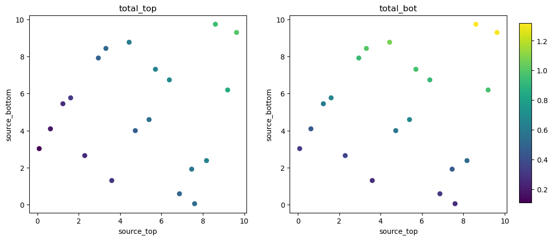
Let’s visualize the training dataset. We scatter the 20 sampled source combinations, coloring them by the target output quantities.
import matplotlib.pyplot as plt

fig, axs = plt.subplots(1, 2, figsize=(12, 5))

for i in range(2):
    plt.sca(axs[i])
    plt.scatter(X[:, 0], X[:, 1], c=Y[:, i], cmap='viridis', vmin=Y.min(), vmax=Y.max())

    plt.title(f'{simulator.output_names[i]}')

    plt.xlabel(f"{simulator.param_names[0]}")
    plt.ylabel(f"{simulator.param_names[1]}")

plt.colorbar(cax=fig.add_axes([0.92, 0.15, 0.02, 0.7]))

plt.show()
Training the surrogate models#
We will train several models by simply instantiating AutoEmulate with our \(X\) and \(Y\) tensors. The library evaluates several typical regression algorithms (like Random Forests, Gaussian Processes, Multi-Layer Perceptrons, etc.) out-of-the-box using the provided data.
from autoemulate import AutoEmulate
# Run AutoEmulate with default settings
ae = AutoEmulate(X, Y, log_level="info")
ae.summarise()
| model_name | x_transforms | y_transforms | params | r2_test | r2_test_std | rmse_test | rmse_test_std | r2_train | r2_train_std | rmse_train | rmse_train_std | |
|---|---|---|---|---|---|---|---|---|---|---|---|---|
| 0 | GaussianProcessMatern32 | [StandardizeTransform()] | [StandardizeTransform()] | {'epochs': 100, 'lr': 0.5, 'likelihood_cls': <... | 1.000000 | 0.000000 | 1.599513e-03 | 8.991597e-04 | 1.000000 | 0.000000 | 2.670971e-04 | 5.090790e-05 |
| 1 | GaussianProcessRBF | [StandardizeTransform()] | [StandardizeTransform()] | {'epochs': 50, 'lr': 0.5, 'likelihood_cls': <c... | 1.000000 | 0.000000 | 9.946671e-04 | 3.879300e-04 | 1.000000 | 0.000000 | 9.191147e-04 | 8.246927e-05 |
| 2 | RadialBasisFunctions | [StandardizeTransform()] | [StandardizeTransform()] | {'kernel': 'thin_plate_spline', 'degree': 1, '... | 1.000000 | 0.000000 | 5.017331e-08 | 1.308012e-08 | 1.000000 | 0.000000 | 3.741635e-08 | 4.359156e-09 |
| 3 | PolynomialRegression | [StandardizeTransform()] | [StandardizeTransform()] | {'lr': 0.1, 'epochs': 500, 'batch_size': 32, '... | 1.000000 | 0.000000 | 2.790703e-08 | 9.141454e-09 | 1.000000 | 0.000000 | 2.814923e-08 | 4.306634e-09 |
| 5 | EnsembleMLP | [StandardizeTransform()] | [StandardizeTransform()] | {'n_emulators': 4, 'epochs': 100, 'layer_dims'... | 0.980582 | 0.079210 | 9.152018e-03 | 4.136176e-03 | 0.999611 | 0.000217 | 4.521532e-03 | 7.270664e-04 |
| 4 | MLP | [StandardizeTransform()] | [StandardizeTransform()] | {'epochs': 200, 'layer_dims': [32, 16], 'lr': ... | 0.964170 | 0.116096 | 8.723211e-03 | 9.216161e-04 | 0.999757 | 0.000192 | 3.577178e-03 | 1.104877e-03 |
Here we decide to select the GaussianProcessRBF model:
# pick GaussianProcessRBF
emulator = [r for r in ae.results if r.model_name == "GaussianProcessRBF"][0]
print(f"Selected model: {emulator.model_name} with id: {emulator.id}")
Selected model: GaussianProcessRBF with id: 1
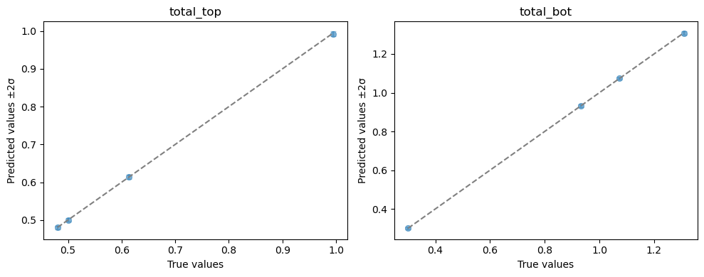
To analyze the emulator’s quality, we plot the predicted versus simulated values on hold-out test data. This is a testing dataset sampled from within the same parameter ranges that was set aside and completely hidden from the surrogate model during its training phase.
Each plotted point represents a single (source_top, source_bottom) input combination. Points closer to the diagonal indicate that the emulator accurately matches the FESTIM high-fidelity predictions.
ae.plot_preds(emulator, output_names=simulator.output_names)
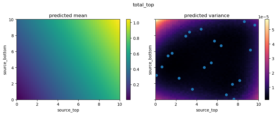
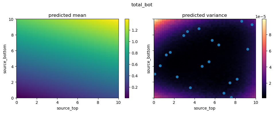
Finally, let’s explore the continuous parameter space by plotting a 2D slice of the surrogate model’s predictions over the source_top and source_bottom space. We can overlay the training samples (points) to see how well the emulator covers the domain.
from autoemulate.core.plotting import create_and_plot_slice

for i in range(2):

    fig, axs = create_and_plot_slice(
        emulator.model,
        output_idx=i,
        parameters_range=simulator.parameters_range,
        quantile=0.5,
        param_pair=(0, 1),
    )
    plt.scatter(X[:, 0], X[:, 1])
    plt.suptitle(f'{simulator.output_names[i]}')
    plt.show()
Performance Comparison#
Finally, we can compare the runtime between executing the full FESTIM physical model and evaluating the trained empirical surrogate using the %timeit notebook magic.
# Time the FESTIM simulator
print("Simulator runtime:")
%timeit simulator.forward(torch.tensor([[5.0, 5.0]]))
Simulator runtime:
10.9 ms ± 148 μs per loop (mean ± std. dev. of 7 runs, 100 loops each)
# Time the empirical surrogate model
print("Emulator runtime:")
%timeit emulator.model.predict(torch.tensor([[5.0, 5.0]]))
Emulator runtime:
2.49 ms ± 38.5 μs per loop (mean ± std. dev. of 7 runs, 100 loops each)
As you can see, substituting FESTIM with the emulator provides a substantial speed-up, highlighting the benefit of training surrogate models in scenarios where a model is evaluated repeatedly (like inference, uncertainty quantification or sensitivity analysis).