Permeation barrier modelling#
In this task, we will model permeation barriers on tungsten and compute the associated Permeation Reduction Factor (PRF).
The PRF is the ratio of the steady state permeation flux without barriers by that of the case with barriers.
Model with barrier#
Let’s first create a model where tungsten is coated with 1 micron of barrier material on both sides.
import festim as F

model_barrier = F.HydrogenTransportProblemDiscontinuous()
/home/docs/checkouts/readthedocs.org/user_builds/festim-workshop/conda/festim2/lib/python3.12/site-packages/festim/coupled_heat_hydrogen_problem.py:1: TqdmExperimentalWarning: Using `tqdm.autonotebook.tqdm` in notebook mode. Use `tqdm.tqdm` instead to force console mode (e.g. in jupyter console)
  import tqdm.autonotebook
Let’s create three VolumeSubdomain1D instances for the three subdomains and assign them to model_barrier.subdomains.
Note
By default, the solubility law of the materials is "sievert".
However, it can be changed by overriding the solubility_law argument to "henry"
barrier_thick = 1e-6
substrate_thick = 3e-3

barrier = F.Material(
    D_0=1e-8,
    E_D=0.39,
    K_S_0=1e22,
    E_K_S=1.04,
)

tungsten = F.Material(
    D_0=4.1e-7,
    E_D=0.39,
    K_S_0=1.87e24,
    E_K_S=1.04,
)

volume_barrier_left = F.VolumeSubdomain1D(
    id=1, borders=[0, barrier_thick], material=barrier
)
volume_tungsten = F.VolumeSubdomain1D(
    id=2, borders=[barrier_thick, substrate_thick + barrier_thick], material=tungsten
)
volume_barrier_right = F.VolumeSubdomain1D(
    id=3,
    borders=[substrate_thick + barrier_thick, substrate_thick + 2 * barrier_thick],
    material=barrier,
)

boundary_left = F.SurfaceSubdomain1D(id=1, x=0)
boundary_right = F.SurfaceSubdomain1D(id=2, x=substrate_thick + 2 * barrier_thick)

model_barrier.subdomains = [
    volume_barrier_left,
    volume_tungsten,
    volume_barrier_right,
    boundary_left,
    boundary_right,
]
model_barrier.surface_to_volume = {
    boundary_left: volume_barrier_left,
    boundary_right: volume_barrier_right,
}

model_barrier.interfaces = [
    F.Interface(id=3, subdomains=[volume_barrier_left, volume_tungsten], penalty_term=1e10),
    F.Interface(id=4, subdomains=[volume_tungsten, volume_barrier_right], penalty_term=1e10),
]
To avoid cells overlapping the domains boundaries, we create 3 lists of vertices.
import numpy as np

vertices_left = np.linspace(0, barrier_thick, num=50)

vertices_mid = np.linspace(barrier_thick, substrate_thick + barrier_thick, num=50)

vertices_right = np.linspace(
    substrate_thick + barrier_thick, substrate_thick + 2 * barrier_thick, num=50
)

vertices = np.concatenate([vertices_left, vertices_mid, vertices_right])

model_barrier.mesh = F.Mesh1D(vertices)
The temperature is homogeneous across the domain.
model_barrier.temperature = 600
A Sievert’s boundary condition is applied on the left surface and the concentration is assumed to be zero on the right surface.
left_bc = F.SievertsBC(
    subdomain=boundary_left, S_0=barrier.K_S_0, E_S=barrier.E_K_S, pressure=100, species=H
)

right_bc = F.FixedConcentrationBC(species=H, subdomain=boundary_right, value=0)

model_barrier.boundary_conditions = [left_bc, right_bc]
For this task, we want to compute the permeation flux, that is the flux at the right surface.
We will also export the concentration profiles at three different times
permeation_flux = F.SurfaceFlux(field=H, surface=boundary_right)

vtx_exports = [
    F.VTXSpeciesExport(filename=f"h_{i}.bp", field=H, subdomain=vol) for i, vol in enumerate(model_barrier.volume_subdomains)
]


profile_exports = [
    F.Profile1DExport(field=spe, subdomain=vol, times=[100, 17000, 8e5])
    for spe in model_barrier.species
    for vol in model_barrier.volume_subdomains
]
model_barrier.exports = [permeation_flux] + vtx_exports + profile_exports
model_barrier.settings = F.Settings(
    atol=1e0,
    rtol=1e-09,
    final_time=8e5,
)


model_barrier.settings.stepsize = F.Stepsize(
    initial_value=5, growth_factor=1.1, cutback_factor=0.9, target_nb_iterations=4, milestones=[100, 17000, 8e5]
)
model_barrier.initialise()
model_barrier.run()
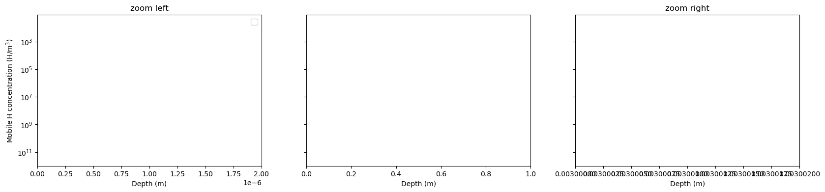
We can plot the concentration profiles at different times and notice the jump of concentrations at interfaces:
/tmp/ipykernel_3258/2865152383.py:23: UserWarning: No artists with labels found to put in legend.  Note that artists whose label start with an underscore are ignored when legend() is called with no argument.
  axs[0].legend(fontsize=12, reverse=True)
Model without barrier#
We can also run the equivalent model without permeation barriers with bare tungsten. Let’s make a few modifications:
model_no_barrier = F.HydrogenTransportProblem()

boundary_left = F.SurfaceSubdomain1D(id=1, x=barrier_thick)
boundary_right = F.SurfaceSubdomain1D(id=2, x=substrate_thick + 1 * barrier_thick)
model_no_barrier.subdomains = [volume_tungsten, boundary_left, boundary_right]

# new mesh
model_no_barrier.mesh = F.Mesh1D(np.linspace(*volume_tungsten.borders, num=50))

# change the solubility of the Sievert's condition
left_bc.S_0 = tungsten.K_S_0
left_bc.E_S = tungsten.E_K_S

model_no_barrier.temperature = model_barrier.temperature
model_no_barrier.boundary_conditions = model_barrier.boundary_conditions
model_no_barrier.species = model_barrier.species

model_no_barrier.settings = model_barrier.settings


permeation_flux_no_barrier = F.SurfaceFlux(field=H, surface=boundary_right)
model_no_barrier.exports = [permeation_flux_no_barrier]

model_no_barrier.initialise()
model_no_barrier.run()
Calculate the PRF#
We can plot the temporal evolution of permeation flux with or without permeation barriers:
import matplotlib.pyplot as plt
plt.figure()

plt.plot(permeation_flux_no_barrier.t, permeation_flux_no_barrier.data, label="without barrier")
plt.plot(permeation_flux.t, permeation_flux.data, label="with barrier")

plt.xscale("log")
plt.legend()
plt.xlabel("Time (s)")
plt.ylabel("Permeation flux (H/m2/s)")
plt.show()
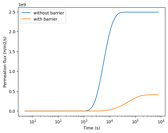
Clearly, having the coating on both sides reduces the permeation flux!
Moreover, it can be shown that the PRF of this configuration is:
With
We can compare the computed PRF to the theory.
computed_PRF = permeation_flux_no_barrier.data[-1] / permeation_flux.data[-1]

diff_ratio = tungsten.D_0 / barrier.D_0
sol_ratio = tungsten.K_S_0 / barrier.K_S_0
length_ratio = barrier_thick / substrate_thick

theoretical_PRF = 1 + 2 * diff_ratio * sol_ratio * length_ratio

print(f"Theoretical PRF = {theoretical_PRF:.4f}")
print(f"Computed PRF = {computed_PRF:.4f}")
print(f"Error = {(computed_PRF - theoretical_PRF)/theoretical_PRF:.2%}")
Theoretical PRF = 6.1113
Computed PRF = 6.0616
Error = -0.81%
Question#
Will adding traps to the simulation change the value of the PRF?
Show solution
No. The PRF is a measure of the flux of mobile particles and is computed at steady state.
At steady state, the McNabb & Foster model states that the concentration of mobile particle is independent of the trapped concentration.
Therefore, the steady state PRF is independent of trapping.