Description

A \(20 \ \mathrm{\mu m}\) thick sample of tungsten was damaged with high energy ions. We estimate the damage region to be \(1 \ \mathrm{\mu m}\) where defects were created.

After the damaging phase, the sample was exposed to energetic D ions for \(2000 \ \mathrm{s}\) at an incident flux of \(5 \ \times 10^{19} \ \mathrm{D \ m^{-2} \ s^{-1} }\) at a temperature \(T_\mathrm{exp} \in [300, 400, 500] \ \mathrm{K}\). We will assume that the implantation follows a gaussian distribution with a mean of \(5 \mathrm{nm}\) and a standard deviation of \(2.1 \ \mathrm{\mu m}\). Moreover, we will assume a reflection coefficient of \(0.5\) (ie. only half the incident ions are implanted).

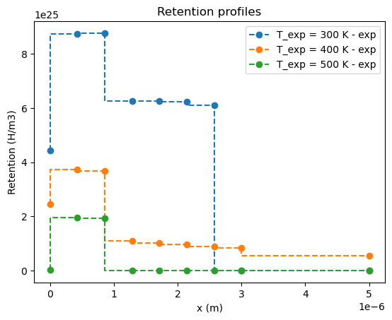
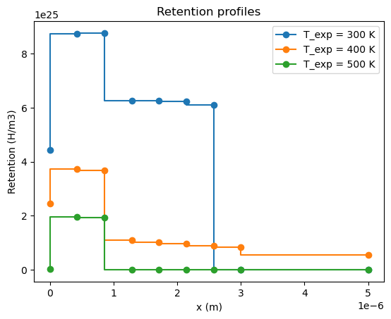
The sample was then stored for approximately \(50 \ \mathrm{s}\) at \(300 \ \mathrm{K}\). After the storage period, Nuclear Reaction Analysis (NRA) was performed to measure the total D concentration profile in the sample up to \(5 \ \mathrm{\mu m}\).

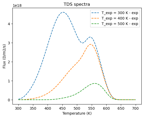
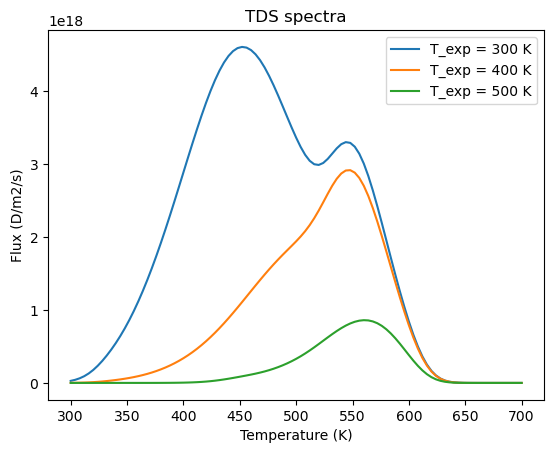
The sample’s temperature was then increased linearly with a ramp of \(4 \ \mathrm{K/s}\) up to \(700 \ \mathrm{K}\) and the desorption flux was measured.

📖 Task: find the set of trapping parameters that reproduce the experimental measurements. You don’t have to simulate the damaging phase.

💡Hint: the damage phase has created traps in the damaged region.

Experimental data

You have access to the experimental TDS measurement and NRA profiles at each exposure temperature. They are stored in challenge_B directory. Each subdirectory contains two txt files retention_profile.txt and tds.txt.

💡 Here are two plotting functions you can use later to plot the experimental data and compare it to your FESTIM script.

import numpy as np
import matplotlib.pyplot as plt


def plot_experimental_tds(T_exp, **kwargs):
    data = np.genfromtxt(f"challenge_B/{T_exp}_K/tds.txt", skip_header=1, delimiter=",")
    flux = data[:, -1]
    tds_T = data[:, 1]
    return plt.plot(tds_T, flux, **kwargs)


def plot_nra_profile(T_exp, **kwargs):
    data = np.genfromtxt(
        f"challenge_B/{T_exp}_K/retention_profile.txt", skip_header=1, delimiter=","
    )
    depth = data[:, 0]
    nra = data[:, 1]
    return plt.step(depth, nra, **kwargs)

Matplotlib is building the font cache; this may take a moment.

exposure_temps = [300, 400, 500]  # K

for T_exp in exposure_temps:
    plot_experimental_tds(T_exp, label=f"T_exp = {T_exp} K")

plt.title("TDS spectra")
plt.xlabel("Temperature (K)")
plt.ylabel("Flux (D/m2/s)")
plt.legend()
plt.show()

for T_exp in exposure_temps:
    plot_nra_profile(T_exp, label=f"T_exp = {T_exp} K", marker="o")

plt.title("Retention profiles")
plt.xlabel("x (m)")
plt.ylabel("Retention (H/m3)")
plt.legend()
plt.show()

import h_transport_materials as htm

# tungsten properties
diffusivity_tungsten = htm.diffusivities.filter(
    material=htm.TUNGSTEN, author="frauenfelder"
)[0]
print(f"Diffusivity of tungsten: \n {diffusivity_tungsten}")

---------------------------------------------------------------------------
ModuleNotFoundError                       Traceback (most recent call last)
Cell In[3], line 1
----> 1 import h_transport_materials as htm
      2 
      3 # tungsten properties
      4 diffusivity_tungsten = htm.diffusivities.filter(

File ~/checkouts/readthedocs.org/user_builds/festim-workshop/conda/festim1/lib/python3.11/site-packages/h_transport_materials/__init__.py:25
     22 Rg = 8.314 * ureg.Pa * ureg.m**3 * ureg.mol**-1 * ureg.K**-1
     23 avogadro_nb = 6.022e23 * ureg.particle * ureg.mol**-1
---> 25 from pybtex.database import parse_file
     26 from pathlib import Path
     28 bib_database = parse_file(str(Path(__file__).parent) + "/references.bib")

File ~/checkouts/readthedocs.org/user_builds/festim-workshop/conda/festim1/lib/python3.11/site-packages/pybtex/database/__init__.py:44
     42 from pybtex.errors import report_error
     43 from pybtex.py3compat import fix_unicode_literals_in_doctest, python_2_unicode_compatible
---> 44 from pybtex.plugin import find_plugin
     47 # for python2 compatibility
     48 def indent(text, prefix):

File ~/checkouts/readthedocs.org/user_builds/festim-workshop/conda/festim1/lib/python3.11/site-packages/pybtex/plugin/__init__.py:26
      2 # Copyright (c) 2006-2021  Andrey Golovizin
      3 # Copyright (c) 2014  Matthias C. M. Troffaes
      4 #
   (...)     21 # TORT OR OTHERWISE, ARISING FROM, OUT OF OR IN CONNECTION WITH THE
     22 # SOFTWARE OR THE USE OR OTHER DEALINGS IN THE SOFTWARE.
     25 import os.path  # splitext
---> 26 import pkg_resources
     28 from pybtex.exceptions import PybtexError
     31 class Plugin(object):

ModuleNotFoundError: No module named 'pkg_resources'

Your answer

implantation_time = 2000  # s
temperature_ramp = 4  # K/s

storage_time = 50  # s
storage_temp = 300  # K

start_tds = implantation_time + storage_time  # s  DON'T RENAME THIS

import festim as F


def festim_model(T_exp):
    """Runs a festim model and returns the derived quantities

    Args:
        T_exp (float): exposure temperature in K

    Returns:
        F.DerivedQuantities: the derived quantities
    """

    # YOUR CODE GOES HERE ...

    derived_quantities = F.DerivedQuantities()

    # ------- YOUR CODE ENDS HERE -------
    return derived_quantities

Here are two plotting functions to plot a simulated TDS spectrum and a simulated retention profile.

def plot_simulated_tds(derived_quantities, **kwargs):
    """Function to plot a simulated TDS spectrum

    Args:
        derived_quantities (festim.DerivedQuantities): the derived quantities object from the simulation.
            Assumes we have an AverageVolume(field="T") and two SurfaceFlux(fields="solute") for surfaces 1 and 2.
        **kwargs: keyword arguments to be passed to the plot function.
    """
    if derived_quantities == []:
        return
    t = np.array(derived_quantities.t)
    indexes = np.where(t >= start_tds)[0]
    temp = np.array(derived_quantities.filter(fields="T").data)
    flux_left = np.array(derived_quantities.filter(fields="solute", surfaces=1).data)
    flux_right = np.array(derived_quantities.filter(fields="solute", surfaces=2).data)

    flux_total = -flux_left - flux_right

    temp = temp[indexes]
    flux_total = flux_total[indexes]
    t = t[indexes]

    return plt.plot(temp, flux_total, **kwargs)


def plot_simulated_profile(filename: str = "", **kwargs):
    if filename == "":
        return
    data_retention = np.genfromtxt(filename, delimiter=",", skip_header=1)
    return plt.plot(data_retention[:, 0], data_retention[:, 1], **kwargs)

We will store all the model results in a dictionary T_exp_to_derived_quantities to be able to retrieve them later.

T_exp_to_derived_quantities = {}

for T_exp in exposure_temps:
    print(f"Running for {T_exp} K")
    derived_quantities = festim_model(T_exp)
    T_exp_to_derived_quantities[T_exp] = derived_quantities

Running for 300 K
Running for 400 K
Running for 500 K

for T_exp in exposure_temps:

    derived_quantities = T_exp_to_derived_quantities[T_exp]

    plt.figure(1)
    (l,) = plot_experimental_tds(
        T_exp, label=f"T_exp = {T_exp} K - exp", linestyle="dashed"
    )
    plot_simulated_tds(
        derived_quantities=derived_quantities, color=l.get_color(), label=f"FESTIM"
    )

    plt.figure(2)
    filename = ""  # CHANGE THIS
    (l,) = plot_nra_profile(
        T_exp, label=f"T_exp = {T_exp} K - exp", linestyle="dashed", marker="o"
    )
    plot_simulated_profile(filename, color=l.get_color(), label=f"FESTIM")

plt.figure(1)
plt.title("TDS spectra")
plt.xlabel("Temperature (K)")
plt.ylabel("Flux (D/m2/s)")
plt.legend()

plt.figure(2)
plt.title("Retention profiles")
plt.xlabel("x (m)")
plt.ylabel("Retention (H/m3)")
plt.legend()

plt.show()