
TDS simulation#
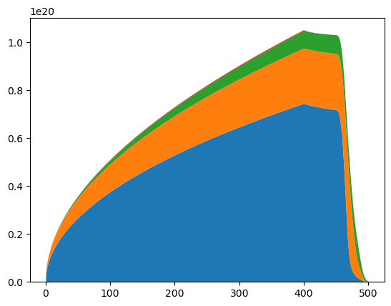
Thermo-desorption spectra (TDS) are a valuble source of experimental data for understanding the mechanics of hydrogen transport. The nature of the spectra produced by thermo-desorption experiments can give insight to the trapping properties of a given material. There are three stages in a TDS experiment; The implantation stage, the resting stage and the desorption stage. Each stage can be modelled, and the desportion flux spectra reproduced.
In this task, we’ll simulate a thermo-desorption experiment for a sample of tungsten.
Objectives
Make a locally refined 1D mesh
Define several traps
Add a time-dependent temperature
Accelerate simulations with adaptive timestepping
Understand the concept of derived quantities
Perform post-processing of derived quantities with
matplotlib
import festim as F
my_model = F.Simulation()
Let’s create a mesh from a list of vertices with more refinement close to \(x=0\).
import numpy as np

vertices = np.concatenate([
    np.linspace(0, 30e-9, num=200),
    np.linspace(30e-9, 3e-6, num=300),
    np.linspace(3e-6, 20e-6, num=200),
])

my_model.mesh = F.MeshFromVertices(vertices)
The material we want to simulate is tungsten. The only property we need is the diffusion coefficient.
tungsten = F.Material(
    id=1,
    D_0=4.1e-07,  # m2/s
    E_D=0.39,  # eV
)

my_model.materials = tungsten
The source term is defined as:
where \(\varphi =2.5 \times 10^{19} \text{m}^{-2}\text{s}^{-1}\) and \(f(x)\) is a Gaussian spatial distribution with a mean value of \(4.5 \: \text{nm}\) and a width of \(2.5 \: \text{nm}\).
FESTIM has a special class for this case: ImplantationFlux.
The ion flux is temporally defined using a Sympy Piecewise expression, to be active for the implantation_time.
Below, t is a built-in FESTIM variable that represent time in \(\text{s}\).
import sympy as sp

implantation_time = 400  # s

ion_flux = sp.Piecewise((2.5e19, F.t <= implantation_time), (0, True))

source_term = F.ImplantationFlux(
    flux=ion_flux,  # H/m2/s
    imp_depth=4.5e-9,  # m
    width=2.5e-9,  # m
    volume=1
)

my_model.sources = [source_term]
/home/docs/checkouts/readthedocs.org/user_builds/festim-workshop/conda/festim1/lib/python3.11/site-packages/mpmath/libmp/libintmath.py:75: DeprecationWarning: bitcount function is deprecated
  warnings.warn("bitcount function is deprecated",
/home/docs/checkouts/readthedocs.org/user_builds/festim-workshop/conda/festim1/lib/python3.11/site-packages/mpmath/libmp/libintmath.py:75: DeprecationWarning: bitcount function is deprecated
  warnings.warn("bitcount function is deprecated",
/home/docs/checkouts/readthedocs.org/user_builds/festim-workshop/conda/festim1/lib/python3.11/site-packages/mpmath/libmp/libintmath.py:75: DeprecationWarning: bitcount function is deprecated
  warnings.warn("bitcount function is deprecated",
/home/docs/checkouts/readthedocs.org/user_builds/festim-workshop/conda/festim1/lib/python3.11/site-packages/mpmath/libmp/libintmath.py:75: DeprecationWarning: bitcount function is deprecated
  warnings.warn("bitcount function is deprecated",
/home/docs/checkouts/readthedocs.org/user_builds/festim-workshop/conda/festim1/lib/python3.11/site-packages/mpmath/libmp/libintmath.py:75: DeprecationWarning: bitcount function is deprecated
  warnings.warn("bitcount function is deprecated",
/home/docs/checkouts/readthedocs.org/user_builds/festim-workshop/conda/festim1/lib/python3.11/site-packages/mpmath/libmp/libintmath.py:75: DeprecationWarning: bitcount function is deprecated
  warnings.warn("bitcount function is deprecated",
/home/docs/checkouts/readthedocs.org/user_builds/festim-workshop/conda/festim1/lib/python3.11/site-packages/mpmath/libmp/libintmath.py:75: DeprecationWarning: bitcount function is deprecated
  warnings.warn("bitcount function is deprecated",
/home/docs/checkouts/readthedocs.org/user_builds/festim-workshop/conda/festim1/lib/python3.11/site-packages/mpmath/libmp/libintmath.py:75: DeprecationWarning: bitcount function is deprecated
  warnings.warn("bitcount function is deprecated",
/home/docs/checkouts/readthedocs.org/user_builds/festim-workshop/conda/festim1/lib/python3.11/site-packages/mpmath/libmp/libintmath.py:75: DeprecationWarning: bitcount function is deprecated
  warnings.warn("bitcount function is deprecated",
/home/docs/checkouts/readthedocs.org/user_builds/festim-workshop/conda/festim1/lib/python3.11/site-packages/mpmath/libmp/libintmath.py:75: DeprecationWarning: bitcount function is deprecated
  warnings.warn("bitcount function is deprecated",
/home/docs/checkouts/readthedocs.org/user_builds/festim-workshop/conda/festim1/lib/python3.11/site-packages/mpmath/libmp/libintmath.py:75: DeprecationWarning: bitcount function is deprecated
  warnings.warn("bitcount function is deprecated",
/home/docs/checkouts/readthedocs.org/user_builds/festim-workshop/conda/festim1/lib/python3.11/site-packages/mpmath/libmp/libintmath.py:75: DeprecationWarning: bitcount function is deprecated
  warnings.warn("bitcount function is deprecated",
/home/docs/checkouts/readthedocs.org/user_builds/festim-workshop/conda/festim1/lib/python3.11/site-packages/mpmath/libmp/libintmath.py:75: DeprecationWarning: bitcount function is deprecated
  warnings.warn("bitcount function is deprecated",
/home/docs/checkouts/readthedocs.org/user_builds/festim-workshop/conda/festim1/lib/python3.11/site-packages/mpmath/libmp/libintmath.py:75: DeprecationWarning: bitcount function is deprecated
  warnings.warn("bitcount function is deprecated",
/home/docs/checkouts/readthedocs.org/user_builds/festim-workshop/conda/festim1/lib/python3.11/site-packages/mpmath/libmp/libintmath.py:75: DeprecationWarning: bitcount function is deprecated
  warnings.warn("bitcount function is deprecated",
/home/docs/checkouts/readthedocs.org/user_builds/festim-workshop/conda/festim1/lib/python3.11/site-packages/mpmath/libmp/libintmath.py:75: DeprecationWarning: bitcount function is deprecated
  warnings.warn("bitcount function is deprecated",
/home/docs/checkouts/readthedocs.org/user_builds/festim-workshop/conda/festim1/lib/python3.11/site-packages/mpmath/libmp/libintmath.py:75: DeprecationWarning: bitcount function is deprecated
  warnings.warn("bitcount function is deprecated",
/home/docs/checkouts/readthedocs.org/user_builds/festim-workshop/conda/festim1/lib/python3.11/site-packages/mpmath/libmp/libintmath.py:75: DeprecationWarning: bitcount function is deprecated
  warnings.warn("bitcount function is deprecated",
In FESTIM, each trap is defined by a Trap object.
Relevent arguments for each trap include:
k_0 and E_k are the trapping rate pre-exponential factor in \(\text{m}^{3} \text{s}^{-1}\) and activation energy in \(\text{eV}\), respectively.
p_0 and E_p are the detrapping rate pre-exponential factor in \(\text{s}^{-1}\) and activation energy in \(\text{eV}\), respectively.
materials is a list of the materials in which the trap is located.
Here, it’s only tungsten.
In FESTIM, traps are intrinsic by default. However, traps can also be implemented as extrinsic, as shown in the example hereafter corresponding to 2 intrinsic and 1 extrinsic trap.
The time evolution of extrinsic traps density \(n_i\) expressed in \(\text{m}^{-3}\) is defined as:
w_atom_density = 6.3e28  # atom/m3

trap_1 = F.Trap(
        k_0=4.1e-7/(1.1e-10**2*6*w_atom_density),
        E_k=0.39,
        p_0=1e13,
        E_p=0.87,
        density=1.3e-3*w_atom_density,
        materials=tungsten
    )
trap_2 = F.Trap(
        k_0=4.1e-7/(1.1e-10**2*6*w_atom_density),
        E_k=0.39,
        p_0=1e13,
        E_p=1.0,
        density=4e-4*w_atom_density,
        materials=tungsten
    )

center = 4.5e-9
width = 2.5e-9
distribution = 1/(width*(2*sp.pi)**0.5) * sp.exp(-0.5*((F.x-center)/width)**2)
trap_3 = F.ExtrinsicTrap(
        k_0=4.1e-7/(1.1e-10**2*6*w_atom_density),
        E_k=0.39,
        p_0=1e13,
        E_p=1.5,
        phi_0=ion_flux,
        n_amax=1e-01*w_atom_density, f_a=distribution, eta_a=6e-4,
        n_bmax=1e-02*w_atom_density, f_b=sp.Piecewise((1e6, F.x < 1e-6), (0, True)), eta_b=2e-4,
        materials=tungsten
    )

my_model.traps = [trap_1, trap_2, trap_3]
Boundary conditions (BCs) can be of several types in FESTIM, the most simple of them being the DirichletBC where an analytical expression is given in the argument: value. The argument surfaces contains a list of all the surfaces on which the BC is applied. If no BC is applied on a surface, it will be considered as a non flux surface (ie \(\frac{\partial c}{\partial\textbf{n}} = 0\)).
In this case, the solute concentration is set to zero on surfaces 1 and 2 (left and right).
my_model.boundary_conditions = [
    F.DirichletBC(surfaces=[1, 2], value=0, field=0)
]
In this example, the temperature is constant from \(t=0\) to \(t=450 \text{s}\) (implantation + resting phase), then increases from \(t=450 \text{s}\) to \(t=500 \text{s}\) in order to perform the thermo-desorption (TDS phase).
\begin{equation} T(t) = \begin{cases} 300, & \text{if} : t < 450 \ 300 + 8(t - 450), & \text{else} \ \end{cases} \end{equation}
\(T\) is expressed in \(\text{K}\).
implantation_temp = 300  # K
temperature_ramp = 8  # K/s

start_tds = implantation_time + 50  # s

my_model.T = sp.Piecewise(
        (implantation_temp, F.t < start_tds),
        (implantation_temp + temperature_ramp*(F.t-start_tds), True))
The Stepsize object defines the simulation stepsize.
The argument initial_value is the initial stepsize is expressed in \(\text{s}\).
An adaptive stepsize algorithm has been implemented in order to save computational cost.
stepsize_change_ratio defines by how much the stepsize is increased or decreased after each iteration (depending on the number of Newton iterations required to converged).
dt_min is the lower limit for the stepsize below which the computation will stop.
The optional argument max_stepsize sets the maximum stepsize. It takes a function of time. In this case, we cap the stepsize at 0.5 s after the start of the TDS.
We also set milestones in order to make sure the simulation doesn’t over step the end of the implantation and the start of the TDS.
my_model.dt = F.Stepsize(
    initial_value=0.5,
    stepsize_change_ratio=1.1,
    max_stepsize=lambda t: 0.5 if t > start_tds else None,
    dt_min=1e-05,
    milestones=[implantation_time, start_tds],
)
my_model.settings = F.Settings(
    absolute_tolerance=1e10,
    relative_tolerance=1e-09,
    final_time=500
)
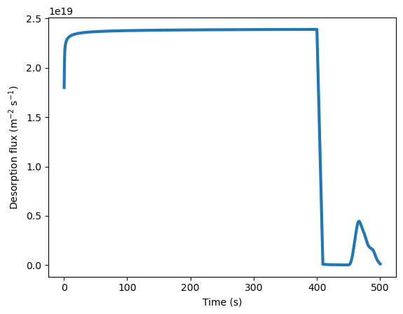
We want to plot the evolution of the surface fluxes as a function of time.
To do so, we’ll use ‘derived quantities’ objects. There is a wide range of derived quantities available in FESTIM.
Here, we’ll use TotalVolume (volume integration) and HydrogenFlux.
list_of_derived_quantities = [
        F.TotalVolume("solute", volume=1),
        F.TotalVolume("retention", volume=1),
        F.TotalVolume("1", volume=1),
        F.TotalVolume("2", volume=1),
        F.TotalVolume("3", volume=1),
        F.HydrogenFlux(surface=1),
        F.HydrogenFlux(surface=2)
    ]

derived_quantities = F.DerivedQuantities(
    list_of_derived_quantities,
    # filename="tds/derived_quantities.csv"  # optional set a filename to export the data to csv
    show_units=True,
)


my_model.exports = [derived_quantities]
my_model.initialise()
my_model.run()
t = derived_quantities.t
flux_left = derived_quantities.filter(fields="solute", surfaces=1).data
flux_right = derived_quantities.filter(fields="solute", surfaces=2).data

flux_total = -np.array(flux_left) - np.array(flux_right)
import matplotlib.pyplot as plt
plt.plot(t, flux_total, linewidth=3)

plt.ylabel(r"Desorption flux (m$^{-2}$ s$^{-1}$)")
plt.xlabel(r"Time (s)")
plt.show()
Make use of numpy to compute the time derivative of the traps inventories!
trap_1 = derived_quantities.filter(fields="1").data
trap_2 = derived_quantities.filter(fields="2").data
trap_3 = derived_quantities.filter(fields="3").data

contribution_trap_1 = -np.diff(trap_1)/np.diff(t)
contribution_trap_2 = -np.diff(trap_2)/np.diff(t)
contribution_trap_3 = -np.diff(trap_3)/np.diff(t)
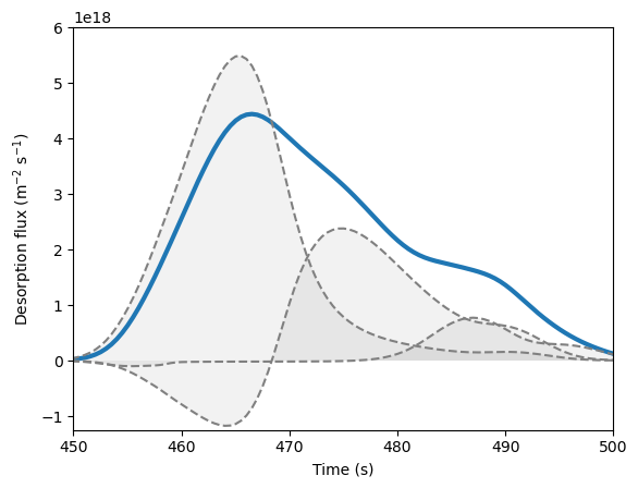
We can now plot the TDS spectrum with the 3 traps contributions
plt.plot(t, flux_total, linewidth=3)
plt.plot(t[1:], contribution_trap_1, linestyle="--", color="grey")
plt.fill_between(t[1:], 0, contribution_trap_1, facecolor='grey', alpha=0.1)
plt.plot(t[1:], contribution_trap_2, linestyle="--", color="grey")
plt.fill_between(t[1:], 0, contribution_trap_2, facecolor='grey', alpha=0.1)
plt.plot(t[1:], contribution_trap_3, linestyle="--", color="grey")
plt.fill_between(t[1:], 0, contribution_trap_3, facecolor='grey', alpha=0.1)

plt.xlim(450, 500)
plt.ylim(bottom=-1.25e18, top=0.6e19)
plt.ylabel(r"Desorption flux (m$^{-2}$ s$^{-1}$)")
plt.xlabel(r"Time (s)")

plt.ylabel(r"Desorption flux (m$^{-2}$ s$^{-1}$)")
plt.xlabel(r"Time (s)")
plt.show()
Task#
Increase the implantation temperature to 500 K and see how the TDS spectrum is affected
Vary the detrapping energy of the first trap
At the end of the implantation phase, what is the proportion of hydrogen trapped in trap 2?