

Write custom classes#
Objectives
Learn how to write custom classes to add more functionality to FESTIM
FESTIM is very flexible. However you may want to customise it further.
You can do this by creating your own classes.
We show here a few examples:
Creating custom derived quantities
Reading the temperature from tabulated data
Add functionalities to the solver
Compute the advection flux#
This example builds upon the previous task Advection-diffusion problem where we obtained a hydrodgen concentration field under the influence of a velocity field.
We would now like to compute the flux \(J\) on the right surface \(\Gamma_\mathrm{right}\) including advection:
where \(v\) is the velocity vector in \(\mathrm{m/s}\), \(c\) is the hydrogen concentration in \(\mathrm{H/m^3}\), and \(\mathbf{n}\) is the outward normal vector.
Just like the advection term in the governing equations, this derived quantity is not natively supported in FESTIM.
It is however possible to make our own DerivedQuantity class to achieve this result.
For more information on class inheritance in python, have a look at this tutorial.
To do so, let’s create a class called SurfaceAdvectionFlux inheriting from festim.SurfaceQuantity.
By doing so, we can inherit from the existing functionalities of the parent class while adding more and overriding the parent class’s behaviour.
This new class will have an argument velocity_field that will take a fenics.Function as value.
This will be stored as an attribute of the class so that we can use it in other methods.
We then add the compute method to compute the correct flux.
import fenics as f
import festim as F


class SurfaceAdvectionFlux(F.SurfaceQuantity):
    def __init__(self, field, surface, velocity_field):

        super().__init__(field=field, surface=surface)

        self.velocity_field = velocity_field
        self.title = "Surface Advection Flux"

    def compute(self):
        # assemble is for integral computation
        # dot is for scalar product
        # n is the normal vector
        # self.function in this case is the concentration
        flux = f.assemble(
            f.dot(
                self.velocity_field * self.function,
                self.n,
            )
            * self.ds(self.surface)
        )
        return flux
Let’s build our model. For details regarding this implementation, have a look at the Advection-diffusion problem task.
from fenics import UnitSquareMesh, CompiledSubDomain, MeshFunction

my_model = F.Simulation()
# creating a mesh with FEniCS
nx = ny = 20
mesh_fenics = UnitSquareMesh(nx, ny)


# marking physical groups (volumes and surfaces)
volume_markers = MeshFunction("size_t", mesh_fenics, mesh_fenics.topology().dim())
volume_markers.set_all(1)

tol = 1e-14

left_surface = CompiledSubDomain("on_boundary && near(x[0], 0, tol)", tol=tol)
right_surface = CompiledSubDomain("on_boundary && near(x[0], 1, tol)", tol=tol)
bottom_surface = CompiledSubDomain("on_boundary && near(x[1], 0, tol)", tol=tol)
top_surface = CompiledSubDomain("on_boundary && near(x[1], 1, tol)", tol=tol)

surface_markers = MeshFunction("size_t", mesh_fenics, mesh_fenics.topology().dim() - 1)
surface_markers.set_all(0)

left_id = 1
top_and_bottom_id = 2
right_id = 3
left_surface.mark(surface_markers, left_id)
right_surface.mark(surface_markers, right_id)
top_surface.mark(surface_markers, top_and_bottom_id)
bottom_surface.mark(surface_markers, top_and_bottom_id)

my_model.mesh = F.Mesh(
    mesh=mesh_fenics, volume_markers=volume_markers, surface_markers=surface_markers
)

my_model.materials = F.Material(id=1, D_0=1, E_D=0)

my_model.T = F.Temperature(500)

my_model.boundary_conditions = [
    F.DirichletBC(field=0, surfaces=top_and_bottom_id, value=0),
    F.DirichletBC(field=0, surfaces=left_id, value=1),
]

my_model.settings = F.Settings(
    absolute_tolerance=1e-10, relative_tolerance=1e-10, transient=False
)

from fenics import interpolate, Expression, VectorFunctionSpace

functionspace = VectorFunctionSpace(my_model.mesh.mesh, "CG", 1)

velocity = Expression(("-100*x[1]*(x[1] - 1)", "0"), degree=2)

velocity = interpolate(velocity, functionspace)
Now we can use our custom derived quantity class and add it to our problem’s exports:
my_model.exports = [
    F.DerivedQuantities(
        [
            SurfaceAdvectionFlux(
                field="solute", surface=right_id, velocity_field=velocity
            )
        ],
        show_units=True,
    )
]
Let’s add the advection term to the governing equations and run the simulation:
from fenics import inner, dot, grad

my_model.initialise()

hydrogen_concentration = my_model.h_transport_problem.mobile.mobile_concentration()
test_function_solute = my_model.h_transport_problem.mobile.test_function

advection_term = (
    inner(dot(grad(hydrogen_concentration), velocity), test_function_solute)
    * my_model.mesh.dx
)

my_model.h_transport_problem.F += advection_term

my_model.run()
We can now compute the flux taking into account the advection field!
flux = my_model.exports[0][0].data[0]
print(f"{flux: .2f} H/m/s")
10.08 H/m/s
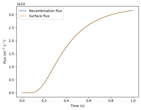
Calculate recombination flux#
Another example is computing the flux of hydrogen \(J\) from:
instead of:
To do so, we can create a custom SurfaceQuantity:
class RecombinationFluxQuantity(F.SurfaceQuantity):
    def __init__(self, Kr_0, E_Kr, order, surface):
        super().__init__(surface=surface, field=0)
        self.Kr_0 = Kr_0
        self.E_Kr = E_Kr
        self.order = order
        self.title = "Recombination flux"

    def compute(self):
        K_r = self.Kr_0 * f.exp(-self.E_Kr / (F.k_B * self.T))
        flux = f.assemble(K_r * self.function**self.order * self.ds(self.surface))
        return flux
import numpy as np

my_model = F.Simulation()
my_model.mesh = F.MeshFromVertices(vertices=np.linspace(0, 7e-5, num=1000))
my_model.materials = F.Material(id=1, D_0=1e-7, E_D=0.2)
my_model.T = F.Temperature(value=700)
my_model.boundary_conditions = [
    F.DirichletBC(surfaces=[1], value=1e15, field=0),
    F.RecombinationFlux(surfaces=[2], Kr_0=1e-15, E_Kr=0.5, order=2),
]
my_model.settings = F.Settings(
    absolute_tolerance=1e8, relative_tolerance=1e-10, final_time=1
)

derived_quantities = F.DerivedQuantities(
    [
        RecombinationFluxQuantity(Kr_0=1e-15, E_Kr=0.5, order=2, surface=2),
        F.SurfaceFlux(field=0, surface=2),
    ],
    show_units=True,
)
my_model.exports = [derived_quantities]


my_model.dt = F.Stepsize(1e-3, stepsize_change_ratio=1.1)

my_model.initialise()

# we just need to teach our custom derived quantity what is the temperature
derived_quantities[0].T = my_model.T.T
my_model.run()
import matplotlib.pyplot as plt
recomb_flux = np.array(derived_quantities[0].data)
surface_flux = -np.array(derived_quantities[1].data)
plt.plot(derived_quantities.t, recomb_flux, label="Recombination flux")
plt.plot(derived_quantities.t, surface_flux, label="Surface flux", linestyle="--")
plt.legend()
plt.xlabel("Time (s)")
plt.ylabel("Flux (m$^{-2}$ s$^{-1}$)")
plt.show()
Temperature from tabulated data#
Using tabulated data for the temperature isn’t natively supported in FESTIM. It doesn’t mean it’s not doable!
Although this requires a bit of FEniCS knowledge, we can extend the Temperature class to make it accept an interpolated object from say scipy.interp1d.
class InterpolatedExpression(f.UserExpression):
def __init__(self, f):
"""InterpolatedExpression
Args:
f (callable): callable y=f(t) that will be used to evaluate the expression
"""
super().__init__()
self.f = f
self.t = 0
def eval(self, value, x):
value[0] = self.f(self.t)
class TemperatureFromData(F.Temperature):
def __init__(self, f):
value = InterpolatedExpression(f)
super().__init__(value)
# override the create_functions method
def create_functions(self, mesh):
"""Creates functions self.T, self.T_n
Args:
mesh (festim.Mesh): the mesh
"""
V = f.FunctionSpace(mesh.mesh, "CG", 1)
self.T = f.Function(V, name="T")
self.T_n = f.Function(V, name="T_n")
self.expression = self.value
self.T.assign(f.interpolate(self.expression, V))
self.T_n.assign(self.T)
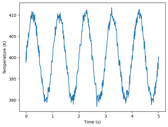
Let’s fabricate some tabulated data:
from scipy.interpolate import interp1d
t = np.linspace(0, 10, num=10000)
T = 400 + 10 * np.sin(2 * np.pi * t)
# add noise
T += np.random.normal(0, 1, size=T.shape)
T_f = interp1d(t, T)
We can then use this new custom temperature class in our model.
my_model = F.Simulation()
my_model.mesh = F.MeshFromVertices(np.linspace(0, 3e-6))
my_model.materials = F.Material(id=1, D_0=1e-7, E_D=0.2)
my_model.T = TemperatureFromData(T_f)
my_model.boundary_conditions = [
F.DirichletBC(surfaces=[1], value=1e15, field=0),
F.DirichletBC(surfaces=[2], value=0, field=0),
]
my_model.settings = F.Settings(
absolute_tolerance=1e10, relative_tolerance=1e-10, transient=True, final_time=5
)
my_model.dt = F.Stepsize(0.0005, stepsize_change_ratio=1.1, max_stepsize=0.01)
my_model.exports = [
F.DerivedQuantities(
[
F.AverageVolume("T", volume=1),
F.SurfaceFlux("0", surface=2),
],
show_units=True,
)
]
my_model.initialise()
my_model.run()
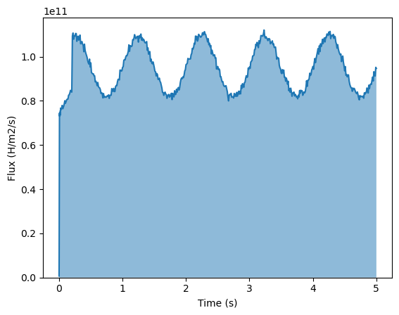
We can see how this noisy temperature affects the desorption flux:
T_t = my_model.exports[0][0].t
T_values = my_model.exports[0][0].data
plt.plot(T_t, T_values)
plt.xlabel("Time (s)")
plt.ylabel("Temperature (K)")
plt.show()
plt.figure()
flux_t = my_model.exports[0][1].t
flux_values = my_model.exports[0][1].data
plt.fill_between(flux_t, np.abs(flux_values), alpha=0.5)
plt.plot(flux_t, np.abs(flux_values))
plt.ylim(bottom=0)
plt.xlabel("Time (s)")
plt.ylabel("Flux (H/m2/s)")
plt.show()
Customise the Simulation class#
The same can be done to add some functionality to the Simulation class. Here, we want to print the number of iterations at the end of the run.
class CustomSimulation(F.Simulation):
def __init__(self, **kwargs):
super().__init__(**kwargs)
self.nb_iterations = 0
def iterate(self):
super().iterate() # do the normal iterate
self.nb_iterations += 1 # count the iterations
def run(self):
super().run() # run the simulation
print(f"Completed in {self.nb_iterations} iterations")
my_model = CustomSimulation()
my_model.mesh = F.MeshFromVertices(np.linspace(0, 3e-6))
my_model.materials = F.Material(id=1, D_0=1e-7, E_D=0.2)
my_model.T = 400
my_model.boundary_conditions = [F.DirichletBC(surfaces=[1], value=1e15, field=0)]
my_model.settings = F.Settings(
absolute_tolerance=1e10, relative_tolerance=1e-10, transient=True, final_time=5
)
my_model.dt = F.Stepsize(1)
my_model.initialise()
my_model.run()
Defining initial values
Defining variational problem
Defining source terms
Defining boundary conditions
Time stepping...
20.0 % 1.0e+00 s Elapsed time so far: 0.0 s
40.0 % 2.0e+00 s Elapsed time so far: 0.0 s
60.0 % 3.0e+00 s Elapsed time so far: 0.0 s
80.0 % 4.0e+00 s Elapsed time so far: 0.0 s
100.0 % 5.0e+00 s Elapsed time so far: 0.0 s
Completed in 5 iterations