Fitting a TDS spectrum

Fitting a TDS spectrum#

Objectives

Use FESTIM to perform some parametric optimisation of thermo-desorption analysis
Learn how FESTIM can be integrated with external python libraries (here scipy.optimize)

In this task, we’ll perform an automated identification of trapping site properties using a parametric optimisation algorithm. See R. Delaporte-Mathurin et al. NME (2021) for more details.

TDS model#

We have to define our FESTIM model, which we’ll use in both task steps. The simulation will be performed for the case of H desorption from a W domain. Using the HTM library, we can get parameters of the H diffusivity in W that are required to set up the model.

import h_transport_materials as htm

D = (
    htm.diffusivities.filter(material="tungsten")
    .filter(isotope="h")
    .filter(author="fernandez")[0]
)
print(D)

---------------------------------------------------------------------------
ModuleNotFoundError                       Traceback (most recent call last)
Cell In[1], line 1
----> 1 import h_transport_materials as htm
      2 
      3 D = (
      4     htm.diffusivities.filter(material="tungsten")

File ~/checkouts/readthedocs.org/user_builds/festim-workshop/conda/festim1/lib/python3.11/site-packages/h_transport_materials/__init__.py:25
     22 Rg = 8.314 * ureg.Pa * ureg.m**3 * ureg.mol**-1 * ureg.K**-1
     23 avogadro_nb = 6.022e23 * ureg.particle * ureg.mol**-1
---> 25 from pybtex.database import parse_file
     26 from pathlib import Path
     28 bib_database = parse_file(str(Path(__file__).parent) + "/references.bib")

File ~/checkouts/readthedocs.org/user_builds/festim-workshop/conda/festim1/lib/python3.11/site-packages/pybtex/database/__init__.py:44
     42 from pybtex.errors import report_error
     43 from pybtex.py3compat import fix_unicode_literals_in_doctest, python_2_unicode_compatible
---> 44 from pybtex.plugin import find_plugin
     47 # for python2 compatibility
     48 def indent(text, prefix):

File ~/checkouts/readthedocs.org/user_builds/festim-workshop/conda/festim1/lib/python3.11/site-packages/pybtex/plugin/__init__.py:26
      2 # Copyright (c) 2006-2021  Andrey Golovizin
      3 # Copyright (c) 2014  Matthias C. M. Troffaes
      4 #
   (...)     21 # TORT OR OTHERWISE, ARISING FROM, OUT OF OR IN CONNECTION WITH THE
     22 # SOFTWARE OR THE USE OR OTHER DEALINGS IN THE SOFTWARE.
     25 import os.path  # splitext
---> 26 import pkg_resources
     28 from pybtex.exceptions import PybtexError
     31 class Plugin(object):

ModuleNotFoundError: No module named 'pkg_resources'

For this task, we’ll consider a simplified simulation scenario. Firstly, we’ll set only one sort of trapping site characterised by a detrapping barrier E_p [eV] and uniformly distributed in the W domain with concentration n [at. fr.]. Secondly, we’ll assume that this W sample was kept in a H environment infinetly long, so all the trap sites were filled with H atoms. Thirdly, we’ll suppose that all mobile H atoms leave the sample before the TDS. Finally, we’ll simulate simulate the TDS phase assuming a uniform heating ramp of 5 K/s.

The initial conditions are: $$ \left.c_{\mathrm{m}}\right\vert_{t=0}=0 $$ \left.c_{\mathrm{t}}\right\vert_{t=0}=n $$ which we’ll set using the InitialCondition class.

For the boundary conditions, we’ll use the assumption of an instantaneous recombination (using DirichletBC): $$ \left.c_{\mathrm{m}}\right\vert_{x=0}=\left.c_{\mathrm{m}}\right\vert_{x=L}=0 $$

For the fitting stage, we have to treat the detrapping energy and the trap concentration as variable parameters. Therefore, we’ll define a function that encapsulates our Simulation object and accepts two input parameters: the trap density and detrapping energy.

import festim as F
import numpy as np

import warnings

warnings.filterwarnings("ignore", category=DeprecationWarning)


def TDS(n, E_p):
    """Runs the simulation with parameters p that represent:

    Args:
        n (float): concentration of trap 1, at. fr.
        E_p (float): detrapping barrier from trap 1, eV

    Returns:
        F.DerivedQuantities: the derived quantities of the simulation
    """
    w_atom_density = 6.3e28  # atom/m3
    trap_conc = n * w_atom_density

    # Define Simulation object
    synthetic_TDS = F.Simulation()

    # Define a simple mesh
    vertices = np.linspace(0, 20e-6, num=200)
    synthetic_TDS.mesh = F.MeshFromVertices(vertices)

    # Define material properties
    tungsten = F.Material(
        id=1,
        D_0=D.pre_exp.magnitude,
        E_D=D.act_energy.magnitude,
    )
    synthetic_TDS.materials = tungsten

    # Define traps
    trap_1 = F.Trap(
        k_0=D.pre_exp.magnitude / (1.1e-10**2 * 6 * w_atom_density),
        E_k=D.act_energy.magnitude,
        p_0=1e13,
        E_p=E_p,
        density=trap_conc,
        materials=tungsten,
    )

    synthetic_TDS.traps = [trap_1]

    # Set initial conditions
    synthetic_TDS.initial_conditions = [
        F.InitialCondition(field="1", value=trap_conc),
    ]

    # Set boundary conditions
    synthetic_TDS.boundary_conditions = [
        F.DirichletBC(surfaces=[1, 2], value=0, field=0)
    ]

    # Define the material temperature evolution
    ramp = 5  # K/s
    synthetic_TDS.T = 300 + ramp * (F.t)

    # Define the simulation settings
    synthetic_TDS.dt = F.Stepsize(
        initial_value=0.01,
        stepsize_change_ratio=1.2,
        max_stepsize=lambda t: None if t < 1 else 1,
        dt_min=1e-6,
    )

    synthetic_TDS.settings = F.Settings(
        absolute_tolerance=1e10,
        relative_tolerance=1e-10,
        final_time=140,
        maximum_iterations=50,
    )

    # Define the exports
    derived_quantities = F.DerivedQuantities(
        [
            F.HydrogenFlux(surface=1),
            F.HydrogenFlux(surface=2),
            F.AverageVolume(field="T", volume=1),
        ]
    )

    synthetic_TDS.exports = [derived_quantities]
    synthetic_TDS.initialise()
    synthetic_TDS.run()

    return derived_quantities

Generate dummy data#

Now we can generate a reference TDS spectrum. For the reference case, we’ll consider the following parameters: $n=0.01~\text{at.fr}$ and $E_p=1~\text{eV}$.

# Get the flux dependence
reference_prms = [1e-2, 1.0]
data = TDS(*reference_prms)

Additionally, we can add some noise to the generated TDS spectra to mimic the experimental conditions. We’ll also save the noisy flux dependence on temperature into a file to use it further as a reference data.

import matplotlib.pyplot as plt

# Get temperature
T = data.filter(fields="T").data

# Calculate the total desorptio flux
flux_left = data.filter(fields="solute", surfaces=1).data
flux_right = data.filter(fields="solute", surfaces=2).data
flux_total = -(np.array(flux_left) + np.array(flux_right))

# Add random noise
noise = np.random.normal(0, 0.05 * max(flux_total), len(flux_total))
noisy_flux = flux_total + noise

# Save to file
np.savetxt(
    "Noisy_TDS.csv", np.column_stack([T, noisy_flux]), delimiter=";", fmt="%f"
)

# Visualise
plt.plot(T, noisy_flux, linewidth=2)

plt.ylabel(r"Desorption flux (m$^{-2}$ s$^{-1}$)")
plt.xlabel(r"Temperature (K)")
plt.show()

---------------------------------------------------------------------------
NameError                                 Traceback (most recent call last)
Cell In[4], line 4
      1 import matplotlib.pyplot as plt
      2 
      3 # Get temperature
----> 4 T = data.filter(fields="T").data
      5 
      6 # Calculate the total desorptio flux
      7 flux_left = data.filter(fields="solute", surfaces=1).data

NameError: name 'data' is not defined

Automated TDS fit#

Here we’ll define the algorithm to fit the generated TDS spectra using the minimize method from the scipy.optimize python library. The initial implementation of the algorithm can be found in this repository. We’ll try to find the values of the detrapping barrier and the trap concetration so the average absolute error between the reference and the fitted spectras satisfies the required tolerance. To start with, we’ll read our reference data and define an auxiliary method to display information on the status of fitting.

ref = np.genfromtxt("Noisy_TDS.csv", delimiter=";")


def info(i, p):
    """
    Print information during the fitting procedure
    """
    print("-" * 40)
    print(f"i = {i}")
    print("New simulation.")
    print(f"Point is: {p}")

---------------------------------------------------------------------------
FileNotFoundError                         Traceback (most recent call last)
Cell In[5], line 1
----> 1 ref = np.genfromtxt("Noisy_TDS.csv", delimiter=";")
      2 
      3 
      4 def info(i, p):

File ~/checkouts/readthedocs.org/user_builds/festim-workshop/conda/festim1/lib/python3.11/site-packages/numpy/lib/_npyio_impl.py:1978, in genfromtxt(fname, dtype, comments, delimiter, skip_header, skip_footer, converters, missing_values, filling_values, usecols, names, excludelist, deletechars, replace_space, autostrip, case_sensitive, defaultfmt, unpack, usemask, loose, invalid_raise, max_rows, encoding, ndmin, like)
   1976     fname = os.fspath(fname)
   1977 if isinstance(fname, str):
-> 1978     fid = np.lib._datasource.open(fname, 'rt', encoding=encoding)
   1979     fid_ctx = contextlib.closing(fid)
   1980 else:

File ~/checkouts/readthedocs.org/user_builds/festim-workshop/conda/festim1/lib/python3.11/site-packages/numpy/lib/_datasource.py:192, in open(path, mode, destpath, encoding, newline)
    155 """
    156 Open `path` with `mode` and return the file object.
    157 
   (...)    188 
    189 """
    191 ds = DataSource(destpath)
--> 192 return ds.open(path, mode, encoding=encoding, newline=newline)

File ~/checkouts/readthedocs.org/user_builds/festim-workshop/conda/festim1/lib/python3.11/site-packages/numpy/lib/_datasource.py:529, in DataSource.open(self, path, mode, encoding, newline)
    526     return _file_openers[ext](found, mode=mode,
    527                               encoding=encoding, newline=newline)
    528 else:
--> 529     raise FileNotFoundError(f"{path} not found.")

FileNotFoundError: Noisy_TDS.csv not found.

Then, we define an error function error_function that:

runs the TDS model with a given set of parameters
calculates the mean absolute error between the reference and the simulated TDS
collects intermediate values of parameters and the calculated errors for visualisation purposes

from scipy.interpolate import interp1d

prms = []
errors = []


def error_function(prm):
    """
    Compute average absolute error between simulation and reference
    """
    global i
    global prms
    global errors
    prms.append(prm)
    i += 1
    info(i, prm)

    # Filter the results if a negative value is found
    if any([e < 0 for e in prm]):
        return 1e30

    # Get the simulation result
    n, Ep = prm
    res = TDS(n, Ep)

    T = np.array(res.filter(fields="T").data)
    flux = -np.array(res.filter(fields="solute", surfaces=1).data) - np.array(
        res.filter(fields="solute", surfaces=2).data
    )

    # Plot the intermediate TDS spectra
    if i == 1:
        plt.plot(T, flux, color="tab:red", lw=2, label="Initial guess")
    else:
        plt.plot(T, flux, color="tab:grey", lw=0.5)

    interp_tds = interp1d(T, flux, fill_value="extrapolate")

    # Compute the mean absolute error between sim and ref
    err = np.abs(interp_tds(ref[:, 0]) - ref[:, 1]).mean()

    print(f"Average absolute error is : {err:.2e}")
    errors.append(err)
    return err

Finally, we’ll minimise error_function to find the set of trap properties reproducing the reference TDS (within some tolerance).

We’ll use the Nelder-Mead minimisation algorithm with the initial guess: $n=0.02~\text{at.fr.}$ and $E_p=1.1~\text{eV}$.

from scipy.optimize import minimize

i = 0  # initialise counter

# Set the tolerances
fatol = 1e18
xatol = 1e-3

initial_guess = [2e-2, 1.1]

# Minimise the error function
res = minimize(
    error_function,
    np.array(initial_guess),
    method="Nelder-Mead",
    options={"disp": True, "fatol": fatol, "xatol": xatol},
)

# Process the obtained results
predicted_data = TDS(*res.x)

T = predicted_data.filter(fields="T").data

flux_left = predicted_data.filter(fields="solute", surfaces=1).data
flux_right = predicted_data.filter(fields="solute", surfaces=2).data
flux_total = -(np.array(flux_left) + np.array(flux_right))

# Visualise
plt.plot(ref[:, 0], ref[:, 1], linewidth=2, label="Reference")
plt.plot(T, flux_total, linewidth=2, label="Optimised")

plt.ylabel(r"Desorption flux (m$^{-2}$ s$^{-1}$)")
plt.xlabel(r"Temperature (K)")
plt.legend()
plt.show()

Show code cell output

Hide code cell output

---------------------------------------------------------------------------
NameError                                 Traceback (most recent call last)
Cell In[7], line 12
      8 
      9 initial_guess = [2e-2, 1.1]
     10 
     11 # Minimise the error function
---> 12 res = minimize(
     13     error_function,
     14     np.array(initial_guess),
     15     method="Nelder-Mead",

File ~/checkouts/readthedocs.org/user_builds/festim-workshop/conda/festim1/lib/python3.11/site-packages/scipy/optimize/_minimize.py:772, in minimize(fun, x0, args, method, jac, hess, hessp, bounds, constraints, tol, callback, options)
    769 callback = _wrap_callback(callback, meth)
    771 if meth == 'nelder-mead':
--> 772     res = _minimize_neldermead(fun, x0, args, callback, bounds=bounds,
    773                                **options)
    774 elif meth == 'powell':
    775     res = _minimize_powell(fun, x0, args, callback, bounds, **options)

File ~/checkouts/readthedocs.org/user_builds/festim-workshop/conda/festim1/lib/python3.11/site-packages/scipy/optimize/_optimize.py:851, in _minimize_neldermead(func, x0, args, callback, maxiter, maxfev, disp, return_all, initial_simplex, xatol, fatol, adaptive, bounds, **unknown_options)
    849 try:
    850     for k in range(N + 1):
--> 851         fsim[k] = func(sim[k])
    852 except _MaxFuncCallError:
    853     pass

File ~/checkouts/readthedocs.org/user_builds/festim-workshop/conda/festim1/lib/python3.11/site-packages/scipy/optimize/_optimize.py:560, in _wrap_scalar_function_maxfun_validation.<locals>.function_wrapper(x, *wrapper_args)
    558 ncalls[0] += 1
    559 # A copy of x is sent to the user function (gh13740)
--> 560 fx = function(np.copy(x), *(wrapper_args + args))
    561 # Ideally, we'd like to a have a true scalar returned from f(x). For
    562 # backwards-compatibility, also allow np.array([1.3]),
    563 # np.array([[1.3]]) etc.
    564 if not np.isscalar(fx):

Cell In[6], line 16, in error_function(prm)
     12     global prms
     13     global errors
     14     prms.append(prm)
     15     i += 1
---> 16     info(i, prm)
     17 
     18     # Filter the results if a negative value is found
     19     if any([e < 0 for e in prm]):

NameError: name 'info' is not defined

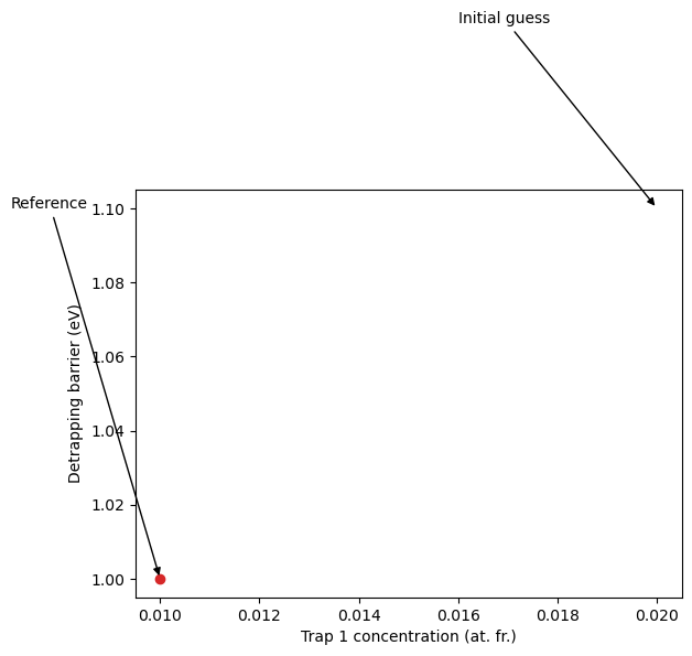
Additionally, we can visualise how the parameters and the computed error varied during the optimisation process.

plt.scatter(
    np.array(prms)[:, 0], np.array(prms)[:, 1], c=np.array(errors), cmap="viridis"
)
plt.plot(np.array(prms)[:, 0], np.array(prms)[:, 1], color="tab:grey", lw=0.5)

plt.scatter(*reference_prms, c="tab:red")
plt.annotate(
    "Reference",
    xy=reference_prms,
    xytext=(reference_prms[0] - 0.003, reference_prms[1] + 0.1),
    arrowprops=dict(facecolor="black", arrowstyle="-|>"),
)
plt.annotate(
    "Initial guess",
    xy=initial_guess,
    xytext=(initial_guess[0] - 0.004, initial_guess[1] + 0.05),
    arrowprops=dict(facecolor="black", arrowstyle="-|>"),
)

plt.xlabel(r"Trap 1 concentration (at. fr.)")
plt.ylabel(r"Detrapping barrier (eV)")
plt.show()

/tmp/ipykernel_5310/1730299763.py:1: UserWarning: No data for colormapping provided via 'c'. Parameters 'cmap' will be ignored
  plt.scatter(

../_images/d8e2b3572b8d85dfd00f9efdc2bcdda42b8e2cb5a2aa7005b92560f20a090c8c.png

Fitting a TDS spectrum

Contents

Fitting a TDS spectrum#

TDS model#

Generate dummy data#

Automated TDS fit#