Advection-diffusion problem

Advection-diffusion problem#

Objectives

Learn how the governing equations can be modified “out-of-the-box”
Simulate an advection-diffusion problem

Natively, advection is not taken into account in FESTIM. The idea is therefore to modify the governing equations by adding an advection term.

Note

Advection terms will be natively supported in FESTIM2!

import festim as F

my_model = F.Simulation()

Create a mesh with FEniCS and mark the subdomains.

For more information on FEniCS meshes, please visit the mesh demo and the subdomains demo.

from fenics import UnitSquareMesh, CompiledSubDomain, MeshFunction, plot

# creating a mesh with FEniCS
nx = ny = 20
mesh_fenics = UnitSquareMesh(nx, ny)


# marking physical groups (volumes and surfaces)
volume_markers = MeshFunction("size_t", mesh_fenics, mesh_fenics.topology().dim())
volume_markers.set_all(1)

tol = 1e-14

left_surface = CompiledSubDomain('on_boundary && near(x[0], 0, tol)',
                                tol=tol)
right_surface = CompiledSubDomain('on_boundary && near(x[0], 1, tol)',
                                     tol=tol)
bottom_surface = CompiledSubDomain('on_boundary && near(x[1], 0, tol)',
                                     tol=tol)
top_surface = CompiledSubDomain('on_boundary && near(x[1], 1, tol)',
                                     tol=tol)

surface_markers = MeshFunction("size_t", mesh_fenics, mesh_fenics.topology().dim() - 1)
surface_markers.set_all(0)

left_id = 1
top_and_bottom_id = 2
right_id = 3
left_surface.mark(surface_markers, left_id)
right_surface.mark(surface_markers, right_id)
top_surface.mark(surface_markers, top_and_bottom_id)
bottom_surface.mark(surface_markers, top_and_bottom_id)

plot(mesh_fenics)

[<matplotlib.lines.Line2D at 0x7cd9943d0cd0>,
 <matplotlib.lines.Line2D at 0x7cd994405f90>]

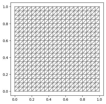
../_images/5e2b023ff229eb4be595c74dac511a6d564838c3fa3f7d8dfd2279b73d126f06.png

The mesh can now be passed to a festim.Mesh instance.

The volume markers and surface markers also need to be passed to the festim.Mesh instance.

my_model.mesh = F.Mesh(
    mesh=mesh_fenics,
    volume_markers=volume_markers,
    surface_markers=surface_markers
)

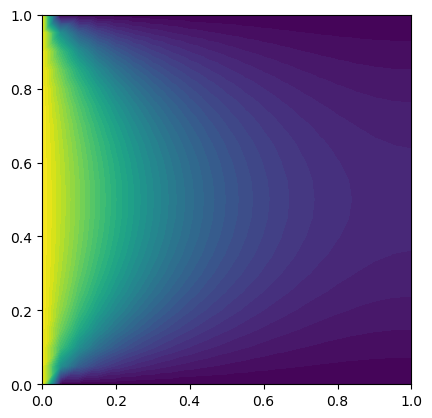
Let’s add the rest of the parameters. For this case, the concentration will be set to 1 on the left surface and to zero on the top and bottom surfaces.

my_model.materials = F.Material(id=1, D_0=1, E_D=0)

my_model.T = 500

my_model.boundary_conditions = [
    F.DirichletBC(field=0, surfaces=top_and_bottom_id, value=0),
    F.DirichletBC(field=0, surfaces=left_id, value=1)
]

my_model.settings = F.Settings(
    absolute_tolerance=1e-10,
    relative_tolerance=1e-10,
    transient=False
    )

We can now run the pure diffusion simulation and visualise the hydrogen concentration field.

my_model.initialise()
my_model.run()

hydrogen_concentration = my_model.h_transport_problem.mobile.solution

plot(hydrogen_concentration)

<matplotlib.tri._tricontour.TriContourSet at 0x7cd987270610>

../_images/fea4af06ea4016e91d9a24b4a9a4f4a564bf89fb92567028c49e9fae43ce5a60.png

Adding advection#

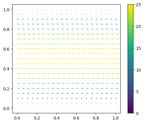
Let’s now add an advection term. To do so, we first need to create a velocity field. For simplicity sake, we will create an arbitrary field velocity.

Note: this velocity field can be obtained from solving the Navier-Stokes equations with FEniCS or with another code (OpenFOAM).

from fenics import interpolate, Expression, VectorFunctionSpace

functionspace = VectorFunctionSpace(my_model.mesh.mesh, "CG", 1)

velocity = Expression(("-100*x[1]*(x[1] - 1)", "0"), degree=2)

velocity = interpolate(velocity, functionspace)

Here’s what velocity looks like:

import matplotlib.pyplot as plt

CS = plot(velocity)
plt.colorbar(CS)
plt.show()

../_images/885ce087dd17db262ab4854e3f0fbf1b0b2fe74c74d62398e1fff0e10fa2f32b.png

Now that we created a FEniCS function representing the velocity, let’s add an advection term to the governing equation.

The governing equation for steady state advection-diffusion is:

\[\nabla \cdot (D \nabla c) - v \cdot \nabla c = 0\]

where \(D\) is the diffusion coefficient, \(c\) is the hydrogen concentration and \(v\) is the velocity.

To modify the governing equations, one needs to modify the formulation of the H transport problem. It can be accessed in my_model.h_transport_problem.F.

See this FEniCS tutorial for more information on finite element formulations.

print(my_model.h_transport_problem.F)

{ (grad(c)) . (grad(v_0)) } * dx(<Mesh #0>[1], {})

from fenics import inner, dot, grad

my_model.initialise() # reinitialisation is needed

hydrogen_concentration = my_model.h_transport_problem.mobile.solution
test_function_solute = my_model.h_transport_problem.mobile.test_function

advection_term = inner(dot(grad(hydrogen_concentration), velocity), test_function_solute) * my_model.mesh.dx

my_model.h_transport_problem.F += advection_term
print(my_model.h_transport_problem.F)

Defining initial values
Defining variational problem
Defining source terms
Defining boundary conditions
{ (grad(c)) . (grad(v_0)) } * dx(<Mesh #0>[1], {})
  +  { (conj((v_0))) * ((grad(c)) . (f_89)) } * dx(<Mesh #0>[everywhere], {})

Now that the governing equation has been modified, let’s run the simulation again and check the new concentration field.

my_model.run()
plot(hydrogen_concentration)
plot(velocity)
plt.show()

Solving steady state problem...
Calling FFC just-in-time (JIT) compiler, this may take some time.

Calling FFC just-in-time (JIT) compiler, this may take some time.

Solved problem in 1.10 s

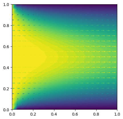
../_images/fd22dbce058278d651f82903beccd78d0219da5a83a6880f77f01b57898e76ae.png

The concentration field is greatly affected as particles are now pushed towards the right hand side of the domain.

Task:#

Vary the velocity field to investigate its influence on the mobile concentration

Advection-diffusion problem

Contents

Advection-diffusion problem#

Adding advection#

Task:#