
Simple simulation#
In this task, we’ll go through the basics of FESTIM and run a simple simulation on a 1D domain.
Objectives
Understand the key building blocks of a FESTIM model
Solve a simple “hello world” problem
The very first step is to import the festim package:
import festim as F

print(F.__version__)
1.4.2
Every FESTIM model is represented by a Simulation object. Here, we give it the name my_model
my_model = F.Simulation()
Several “ingredients” are now required to run a FESTIM simulation:
a mesh
a temperature
a set of materials
optionally: trapping properties
boundary conditions
optionally: sources of H
simulation settings
a stepsize for transient problems
1. Mesh#
FESTIM simulations need a mesh. FESTIM provides support for simple 1D meshes. More complicated meshes can be imported from external software (see Heat transfer simulations).
The most straightforward mesh is MeshFromVertices, which takes a vertices argument.
Here’s a simple mesh with a few vertices:
F.MeshFromVertices(vertices=[0, 1, 2, 3, 4, 5, 6, 7, 7.5])
<festim.meshing.mesh_from_vertices.MeshFromVertices at 0x7b82af7287d0>
Numpy can be used to generate heavier meshes. Here we create a mesh containing 1000 cells over a [0, 7e-6] domain (7 microns).
This mesh is assigned to the simulation by setting the .mesh attribute of my_model.
import numpy as np

my_model.mesh = F.MeshFromVertices(vertices=np.linspace(0, 7e-6, num=1001))
2. Materials#
Material objects hold the materials properties like diffusivity and solubility.
Here we only need the diffusivity defined as an Arrhenius law:
where \(k_B\) is the Boltzmann constant in eV/K and \(T\) is the temperature in K. From this, the pre-exponential coefficient, \(D_0\) in m2/s, and the diffusion actiavtion energy, \(E_D\) in eV are needed.
Note
All units in FESTIM as SI (apart for activation energies that are in eV)
To check what unit is expected by FESTIM, check the documentation. Here is the reference for the Material class
my_model.materials = F.Material(id=1, D_0=1e-7, E_D=0.2)
3. Temperature#
Temperature is a very important parameter in hydrogen transport.
The value can be a simple float (like here 300) or a sympy expression like 500 + 3*sympy.exp(-F.x).
The temperature is in K.
Note
For heat transfer simulations, the HeatTransferProblem can be used instead. See Heat transfer simulations
my_model.T = 300
4. Boundary conditions & source#
Our hydrogen transport problem now needs boundary conditions and a volumetric source term.
FESTIM provides plenty of boundary conditions (see Boundary Conditions).
Here we’ll simply set the mobile concentration at 1e15 on the left and right boundaries (resp. 1 and 2).
fieldrepresents the variable on which the boundary condition is imposed. Here,0stands for the mobile hydrogen concentration.valueis the value of the mobile concentration. Again, it could be a function of time and space with1e15*F.x + F.tsurfacesis a list of surfaces ids (in 1D,1is left and2is right)
A volumetric source of mobile H (field=0) is set in the whole volume (volume=1) and its value is 1e20 H/m3/s.
Additional sources can be applied.
my_model.boundary_conditions = [
    F.DirichletBC(surfaces=[1, 2], value=1e15, field=0)  # H/m3
]


my_model.sources = [F.Source(value=1e20, volume=1, field=0)]  # H/m3/s
5. Settings#
With Settings we set the main solver parameters.
absolute_tolerance: the absolute tolerance of the Newton solver. For concentrations in \(\mathrm{m}^{-3}\),1e10is usually fine.relative_tolerance: the relative tolerance of the Newton solver. Values around1e-10are good practices.final_time: since we want to solve a transient problem, we need to set the final time. Here, 100 s.
Tip
Tuning absolute and relative tolerances can be a fine art. If tolerances the solver may not converge.
If they are too high, the solver may converge to quickly (in zero iterations), resulting in no evolution of the concentration fields.
To have more information on the solving steps, set the log level of the solver to 20 with my_model.log_level = 20 (default is 40)
my_model.settings = F.Settings(
    absolute_tolerance=1e10, relative_tolerance=1e-10, final_time=2  # s
)
6. Exports#
Finally, we want to be able to visualise the concentration field.
To do so, we add an XDMFExport object which will export the concentration field at each timestep to an XDMF file.
This XDMF file can then be read in Paraview.
field: the field we want to export. Here,"solute"stands for the mobile concentration of hydrogen. It could be"retention","1"(trap 1),"T"(temperature)filename: the path to the exported file
Note
For 1D fields, the checkpoint attribute needs to be set to False to be visualised in Paraview. Refer to this issue.
results_folder = "task01"
my_model.exports = [
    F.XDMFExport(
        field="solute",
        filename=results_folder + "/hydrogen_concentration.xdmf",
        checkpoint=False,  # needed in 1D
    ),
    F.TXTExport(
        field="solute",
        times=[0.1, 0.2, 0.5, 1],
        filename=results_folder + "/mobile_concentration.txt",
    ),
]
7. Stepsize#
Since we are solving a transient problem, we need to set a Stepsize.
Here, the value of the stepsize is fixed at 0.05.
We also add milestones to ensure the simulation passes by specific times.
Note
Transient simulations can be accelerated with adaptive stepsize. See Task 2
my_model.dt = F.Stepsize(0.05, milestones=[0.1, 0.2, 0.5, 1]) # s
8. Run#
Finally, we initialise the model and run it!
my_model.initialise()

my_model.run()
Three files should have been created: hydrogen_concentration.xdmf, hydrogen_concentration.h5, and mobile_concentration.txt
The .xdmf file is the one that can be opened in Paraview, and it points to the .h5 file.
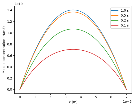
The profile exported as a text file can now be plotted with matplotlib:
import matplotlib.pyplot as plt
import numpy as np
data = np.genfromtxt(
results_folder + "/mobile_concentration.txt", skip_header=1, delimiter=","
)
plt.plot(data[:, 0], data[:, 4], label="1.0 s")
plt.plot(data[:, 0], data[:, 3], label="0.5 s")
plt.plot(data[:, 0], data[:, 2], label="0.2 s")
plt.plot(data[:, 0], data[:, 1], label="0.1 s")
plt.xlabel("x (m)")
plt.ylabel("Mobile concentration (H/m3)")
plt.legend()
plt.show()
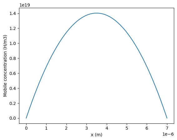
To solve the steady-state problem, simply set:
my_model.settings.transient = False
my_model.dt = None
my_model.exports = [
F.TXTExport(
field="solute", filename=results_folder + "/mobile_concentration_steady.txt"
)
]
my_model.initialise()
my_model.run()
Defining initial values
Defining variational problem
Defining source terms
Defining boundary conditions
Solving steady state problem...
Calling FFC just-in-time (JIT) compiler, this may take some time.
Calling FFC just-in-time (JIT) compiler, this may take some time.
Solved problem in 1.10 s
data = np.genfromtxt(
    results_folder + "/mobile_concentration_steady.txt", skip_header=1, delimiter=","
)

plt.plot(data[:, 0], data[:, 1])
plt.xlabel("x (m)")
plt.ylabel("Mobile concentration (H/m3)")
plt.show()