Active learning

Objectives

• Understand when and why active learning is beneficial for computationally expensive simulators

• Implement an active learning strategy using AutoEmulate’s learner API to iteratively improve a surrogate model

In many real-world scenarios, running a high-fidelity simulator is computationally expensive. Generating a large dataset upfront to train a surrogate model might not be feasible. Active learning addresses this by training an initial model on a small dataset and then iteratively querying the simulator for new data points that provide the most information.

In this tutorial, we will use the AutoEmulate active learning features to iteratively improve a Gaussian Process (GP) emulator for a FESTIM model.

import matplotlib.pyplot as plt
from autoemulate.learners import stream
from autoemulate.emulators import GaussianProcessRBF

Matplotlib is building the font cache; this may take a moment.

The FESTIM Simulator

We will reuse the same 2D FESTIM problem from the previous tutorial. We define a make_model function that creates the unit square geometry with two subdomains, applies two parameters (source_top and source_bottom), and extracts two quantities of interest (total_top and total_bot).

We then wrap this into the FestimProblem inheriting from Simulator.

import festim as F

from dolfinx.mesh import create_unit_square
from mpi4py import MPI
from autoemulate.simulations.base import Simulator
import torch


def make_model(source_bottom: float, source_top: float) -> F.HydrogenTransportProblem:
    fenics_mesh = create_unit_square(MPI.COMM_WORLD, 20, 20)

    festim_mesh = F.Mesh(fenics_mesh)

    material_top = F.Material(D_0=0.2, E_D=0)
    material_bot = F.Material(D_0=0.1, E_D=0)

    top_volume = F.VolumeSubdomain(
        id=1, material=material_top, locator=lambda x: x[1] >= 0.5
    )
    bottom_volume = F.VolumeSubdomain(
        id=2, material=material_bot, locator=lambda x: x[1] <= 0.5
    )

    boundary = F.SurfaceSubdomain(id=1)

    my_model = F.HydrogenTransportProblem()
    my_model.mesh = festim_mesh
    my_model.subdomains = [boundary, top_volume, bottom_volume]

    H = F.Species("H")
    my_model.species = [H]

    my_model.temperature = 400

    my_model.boundary_conditions = [
        F.FixedConcentrationBC(subdomain=boundary, value=0.0, species=H),
    ]

    my_model.sources = [
        F.ParticleSource(species=H, volume=bottom_volume, value=source_bottom),
        F.ParticleSource(species=H, volume=top_volume, value=source_top),
    ]

    my_model.settings = F.Settings(atol=1e-10, rtol=1e-10, transient=False)

    my_model.exports = [
        F.TotalVolume(field=H, volume=top_volume),
        F.TotalVolume(field=H, volume=bottom_volume),
    ]

    return my_model


class FestimProblem(Simulator):
    def __init__(
        self,
        param_ranges={"source_top": (0.0, 10.0), "source_bottom": (0.0, 10.0)},
        output_names=["total_top", "total_bot"],
    ):
        super().__init__(param_ranges, output_names, log_level="error")

    def _forward(self, x: torch.Tensor) -> torch.Tensor:
        source_top = x[:, 0]
        source_bottom = x[:, 1]

        # convert to float
        source_top = source_top.item()
        source_bottom = source_bottom.item()
        model = make_model(source_bottom, source_top)

        # Solve the model
        model.initialise()
        model.run()

        # Extract the total amount of H in the top and bottom volumes
        total_top = model.exports[0].data
        total_bot = model.exports[1].data

        y = torch.tensor([total_top, total_bot]).T
        # Ensure the output is a 2D tensor
        if y.ndim == 1:
            y = y.unsqueeze(1)

        return y

Training an Initial (Weak) Emulator

We will start by training an initial Gaussian Process emulator. Unlike the previous tutorial where we generated a comprehensive dataset, here we intentionally restrict our initial training dataset to only 5 points. This simulates a scenario where generating data is expensive and initial data is scarce.

simulator = FestimProblem()

# Train emulator
x_train = simulator.sample_inputs(5)
y_train, _ = simulator.forward_batch(x_train)


def make_gp(x_train, y_train, lr=5e-2):
    return GaussianProcessRBF(
        x_train,
        y_train,
        lr=lr,
        standardize_y=False,
    )


emulator = make_gp(x_train, y_train)
emulator.fit(x_train, y_train)

# Test emulator
x_test = simulator.sample_inputs(100)
y_mean, var = emulator.predict_mean_and_variance(x_test)
y_std = var.sqrt()
y_true, _ = simulator.forward_batch(x_test)

We can plot the 2D parameter space using the create_and_plot_slice function. Since the emulator was trained on only 5 random points, its predictions are likely to be inaccurate across the wider parameter space.

from autoemulate.core.plotting import create_and_plot_slice

for i in range(2):
    fig, axs = create_and_plot_slice(
        emulator,
        output_idx=i,
        parameters_range=simulator.parameters_range,
        quantile=0.5,
        param_pair=(0, 1),
    )
    plt.scatter(x_train[:, 0], x_train[:, 1])
    plt.suptitle(f"{simulator.output_names[i]}")
    plt.show()

Setting up the Active Learner

To improve our emulator effectively without blindly sampling everywhere, we will use AutoEmulate’s active learning API. We set up the untrained emulator as a starting point and initialize a stream.Random learner.

This learner will sequentially analyze points from an input stream and evaluate whether each new point should be simulated and added to the training set based on an exploration probability (p_query). In more complex scenarios, you could use advanced algorithms like Uncertainty sampling where the model queries where it’s most unconfident.

x_train = simulator.sample_inputs(5)
y_train, _ = simulator.forward_batch(x_train)
emulator = make_gp(x_train, y_train, 0.1)

# Learner
learner = stream.Random(
    simulator=simulator,
    emulator=emulator,
    x_train=x_train,
    y_train=y_train,
    p_query=0.2,
    show_progress=False,
)

# Stream samples
X_stream = simulator.sample_inputs(100)
learner.fit_samples(X_stream)

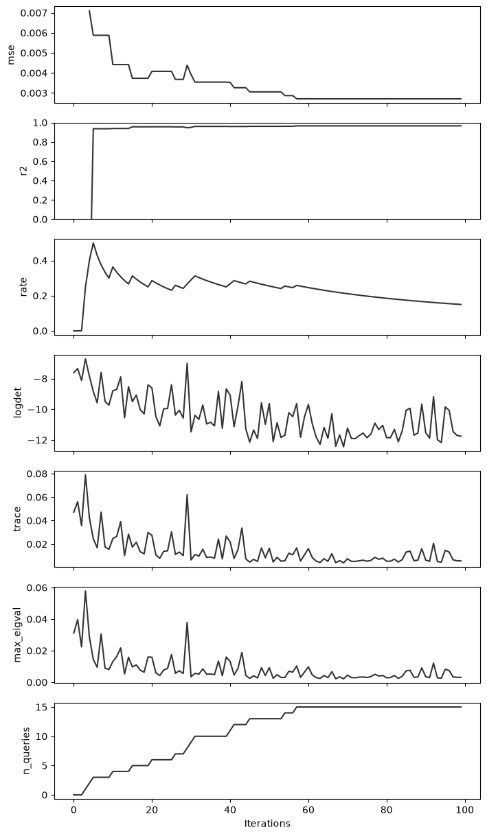
Model Evaluation

The Learner records various regression metrics during the stream evaluation, such as Mean Squared Error (MSE) and R² score. We can plot these metrics vs iteration count to objectively observe the emulator learning dynamically.

fig, axs = plt.subplots(
    nrows=len(learner.metrics), ncols=1, sharex=True, figsize=(8, 15)
)
for i, (k, v) in enumerate(learner.metrics.items()):
    axs[i].plot(v, c="k", alpha=0.8)
    axs[i].set_ylabel(k)
axs[-1].set_xlabel("Iterations")

axs[1].set_ylim(0, 1)
plt.show()

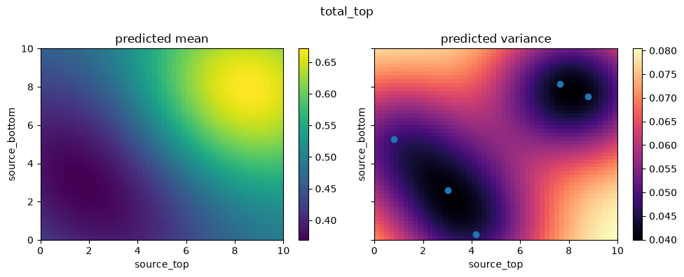
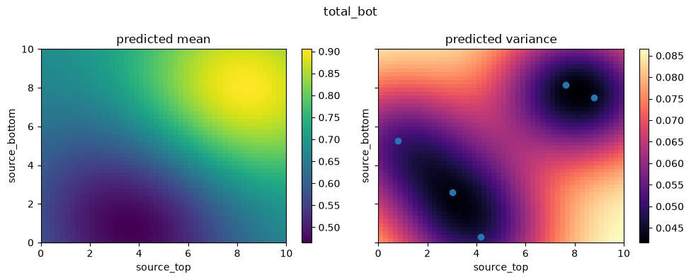
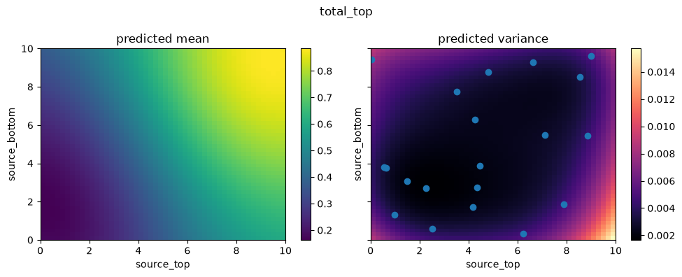
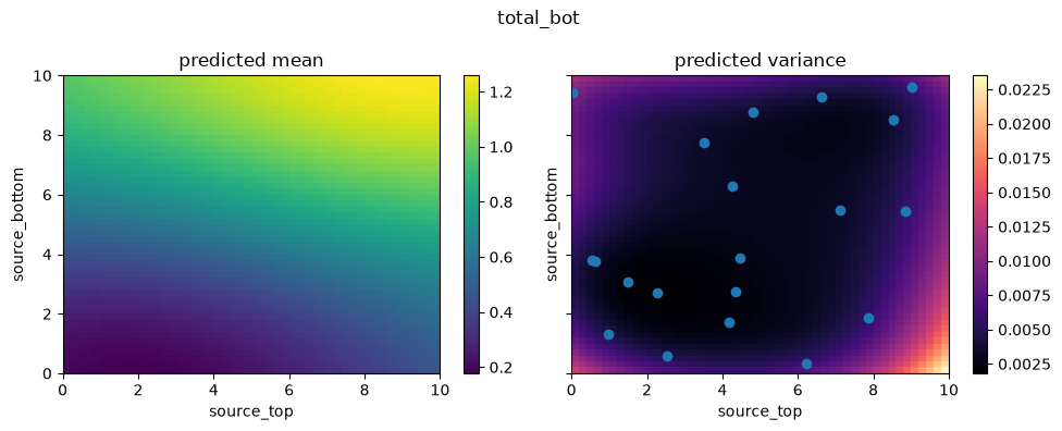
Let’s visualize the 2D parameter space again. This time, we plot slices using the updated emulator currently stored inside the learner.emulator, which has continually trained itself using the actively sampled points.

You should notice a drastically smoother, more accurate response mapping compared to the previous slice with 5 points.

for i in range(2):
    fig, axs = create_and_plot_slice(
        learner.emulator,
        output_idx=i,
        parameters_range=simulator.parameters_range,
        quantile=0.5,
        param_pair=(0, 1),
    )
    plt.scatter(learner.x_train[:, 0], learner.x_train[:, 1])
    plt.suptitle(f"{simulator.output_names[i]}")
    plt.show()

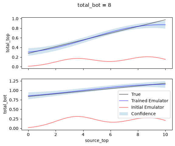
To investigate more clearly the advantage acquired by active learning, we can sample a continuous 1D line slice through our parameters (e.g. fixing the bottom source rate equal to 8).

In the plot below, we compare:

1. The real underlying simulations (True values).

2. The Initial Emulator that was trained on 5 points (red).

3. The Predicted values spanning out of our actively learned surrogate model.

value_to_fix = 8

x_line = torch.linspace(0, 10, 100).unsqueeze(1)
y_line = torch.full_like(x_line, value_to_fix)

x_line = torch.cat([x_line, y_line], dim=1)

# true values along the line
y_line_true, _ = simulator.forward_batch(x_line)

predicted_mean, var = learner.emulator.predict_mean_and_variance(x_line)
predicted_std = var.sqrt()

predicted_mean_old, var_old = emulator.predict_mean_and_variance(x_line)
predicted_std_old = var_old.sqrt()

# plot
fig, axs = plt.subplots(nrows=2, ncols=1, sharex=True)
for i in range(2):
    plt.sca(axs[i])
    plt.plot(x_line[:, 0], y_line_true[:, i], label="True", c="k", alpha=0.5)
    plt.plot(x_line[:, 0], predicted_mean[:, i], label="Trained Emulator", c="b", alpha=0.5)
    plt.plot(
        x_line[:, 0],
        predicted_mean_old[:, i],
        label="Initial Emulator",
        c="r",
        alpha=0.5,
    )
    plt.fill_between(
        x_line[:, 0],
        predicted_mean[:, i] - predicted_std[:, i],
        predicted_mean[:, i] + predicted_std[:, i],
        alpha=0.2,
        label="Confidence",
    )
    plt.ylabel(simulator.output_names[i])

plt.suptitle(f"{simulator.output_names[i]} = {value_to_fix}")
plt.xlabel(simulator.param_names[0])
plt.legend()
plt.show()