Visualizing fields in ParaView

ParaView is a strong visualization tool that users can use to view their FESTIM exports. This tutorial goes over a simple introduction to viewing results in ParaView.

Take a look at ParaView’s download page for more information on installing ParaView, or ParaView’s user guide to learn more about using ParaView.

Objectives:

• Creating a VTX species export

• Opening export in ParaView

• Learn additional helpful functionalities

Creating a VTX species export

First, let us run a simple 2D diffusion problem and export a VTX file:

Show code cell source

Hide code cell source

import festim as F
import numpy as np
from dolfinx.mesh import create_unit_square
from mpi4py import MPI

fenics_mesh = create_unit_square(MPI.COMM_WORLD, 10, 10)
festim_mesh = F.Mesh(fenics_mesh)

my_model = F.HydrogenTransportProblem()

mat = F.Material(D_0=1, E_D=0)

vol = F.VolumeSubdomain(id=1, material=mat)
top_surface = F.SurfaceSubdomain(id=1, locator=lambda x: np.isclose(x[1], 1.0))
bottom_surface = F.SurfaceSubdomain(id=2, locator=lambda x: np.isclose(x[1], 0.0))

my_model.mesh = festim_mesh
my_model.subdomains = [top_surface, bottom_surface, vol]

H = F.Species("H")
my_model.species = [H]
my_model.temperature = 400

my_model.boundary_conditions = [
    F.FixedConcentrationBC(subdomain=top_surface, value=1.0, species=H),
    F.FixedConcentrationBC(subdomain=bottom_surface, value=0.0, species=H),
]

my_model.exports = [
    F.VTXSpeciesExport(filename="paraview/out.bp",field=H,subdomain=vol,checkpoint=False)
]

my_model.settings = F.Settings(atol=1e-10, rtol=1e-10, transient=False)

my_model.initialise()
my_model.run()

/home/docs/checkouts/readthedocs.org/user_builds/festim-workshop/conda/latest/lib/python3.12/site-packages/festim/coupled_heat_hydrogen_problem.py:1: TqdmExperimentalWarning: Using `tqdm.autonotebook.tqdm` in notebook mode. Use `tqdm.tqdm` instead to force console mode (e.g. in jupyter console)
  import tqdm.autonotebook

We should expect to see a new folder created named paraview/out.bp.

Opening file in ParaView

Now, we can open ParaView and open our exported file.

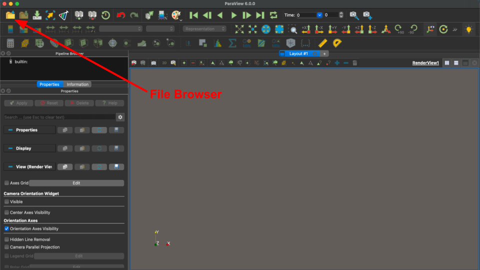
First, we need to select the correct file by navigating to the file browser located in the top left:

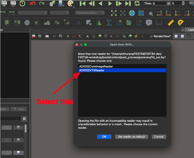
If this is the first time you open a .bp file in ParaView, you may be prompted to select a suitable reader. Be sure to select ADIOS2VTXReader, otherwise you will not be able to view the export and ParaView may crash (see image below):

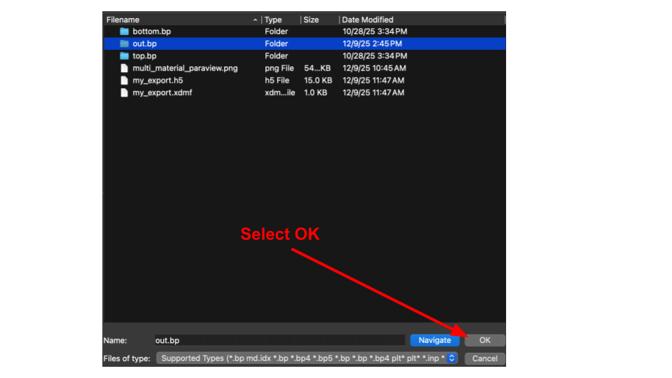
Then, we select our out.bp file and press OK on the bottom:

Now we must press apply to visualize our domain:

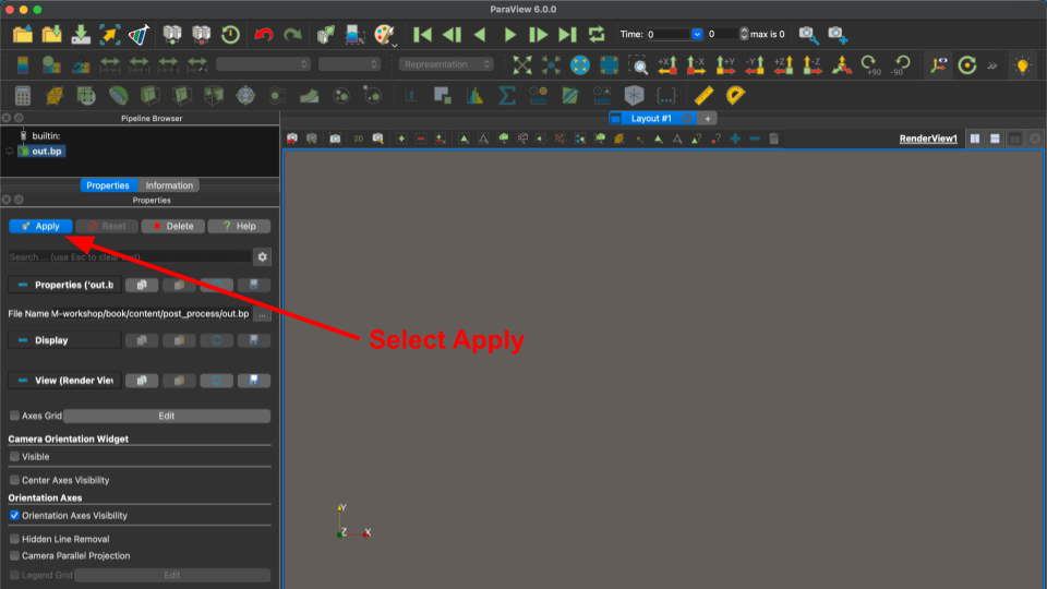
Note

To view the export in ParaView, you must click apply to the .bp folder. If you try to open the .bp folder and select one of the files, you will not be able to view your export.

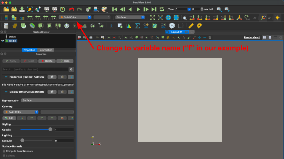
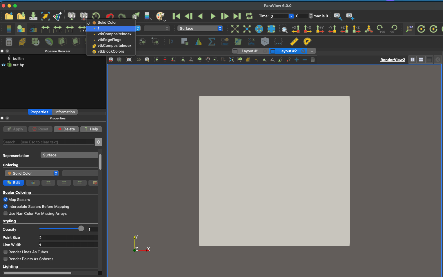
To view our concentration, we need to select the dropdown box that says “Solid Color” and change it to our field variable (named “f” in our example):

Tip

Users can also choose to view other exported fields (such as temperature) using this dropdown section.

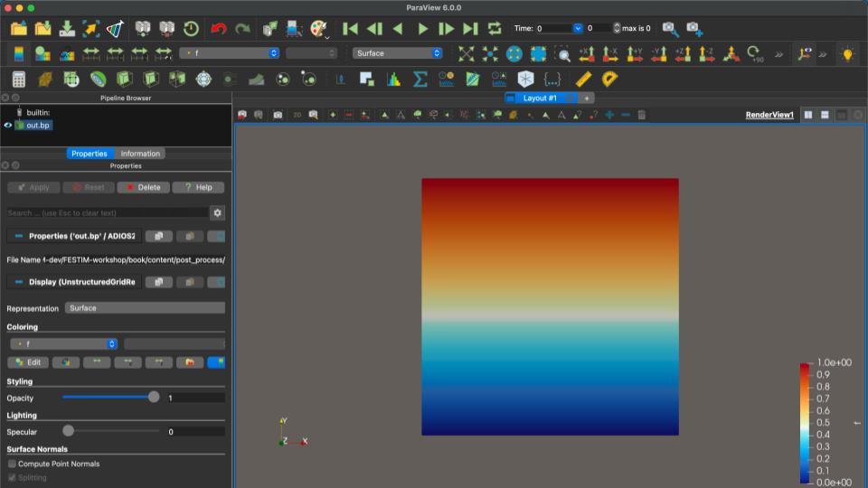
Finally, we see our diffusion field!

Learn additional helpful functionalities

It may be helpful to utilize some other functionalities in ParaView. Here we discuss some commonly used ones.

Viewing results from a 1D simulation

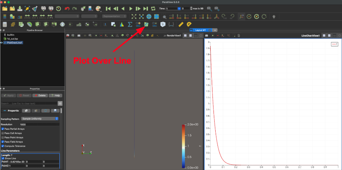
Users can view results from a 1D FESTIM simulation using Plot Over Line.

Let’s run a simple 1D, transient diffusion simulation and export a 1D profile named paraview/1d_out.bp:

Show code cell source

Hide code cell source

import festim as F
import numpy as np

my_model = F.HydrogenTransportProblem()
my_model.mesh = F.Mesh1D(vertices=np.linspace(0, 1, num=1001))
mat = F.Material(D_0=1e-3, E_D=0)
volume_subdomain = F.VolumeSubdomain1D(id=1, borders=[0, 1], material=mat)
boundary_left = F.SurfaceSubdomain1D(id=1, x=0)
boundary_right = F.SurfaceSubdomain1D(id=2, x=1)
my_model.subdomains = [volume_subdomain, boundary_left, boundary_right]
my_model.temperature = 300
H = F.Species("H")
my_model.species = [H]

my_model.boundary_conditions = [
    F.FixedConcentrationBC(subdomain=boundary_left, value=2, species=H),
    F.FixedConcentrationBC(subdomain=boundary_right, value=0, species=H),
]


my_model.exports = [F.VTXSpeciesExport(filename="paraview/1d_out.bp", field=H)]
my_model.settings = F.Settings(atol=1e-10, rtol=1e-10, stepsize=1,final_time=100) 

my_model.initialise()
my_model.run()

When we open the export in ParaView, we can click on the Plot Over Line option, which will show a plot of the concentration versus mesh position, as shown below:

Note

If users exported a 1D transient result into ParaView, you can plot the 1D profile first, and then click Play to see the profile change over time. See more information about time controls below.

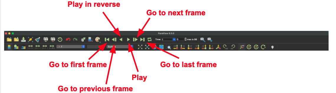
Utilizing time controls

For transient solutions, users can utilize the time controls given in the tool bar:

Scaling data ranges and changing colorbars

It may be necessary to re-scale data ranges over different exports or timesteps. To do this, users can select one of the options shown below:

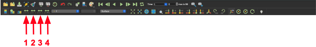
Here’s a quick summary of each option’s functionality:

• 1 (Rescale to data range): Sets the minimum/maximum from the current timestep

• 2 (Rescale to custom data range): Manually set the minimum and maximum values

• 3 (Rescale to data range over all timestep): Sets the minimum/maximum by parsing through all timesteps

• 4 (Rescale to visible data range): Sets minumum and maximum from visible objects this timestep

The colormap will adjust accordingly to the rescaled data.

Users can also change the color bar by selecting Edit Color Map and then selecting a color map from the dropdown menu, as shown below:

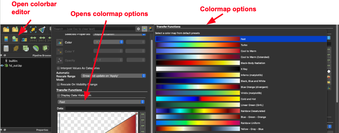
Learn more about color maps and palettes here.

Slicing your results when using 3D data

Users may want to view a 2D result of a 3D solution, which can be done using the Clip or Slice options. Clipping will show a 3D volume that is sectioned by a specified plane, while slicing will prduce a 2D plane of data using a reference plane. For 3D data exports, it is almost always necessary to use clipping or slicing to for field visualization.

Let us run a steady-state, 3D example with the following boundary conditions:

\[ \text{Bottom surface:} \quad \mathrm{c} = 1 \]

\[ \text{Top and side surfaces:} \quad \mathrm{c} = 0 \]

Show code cell source

Hide code cell source

from dolfinx.mesh import create_unit_cube
from mpi4py import MPI
import festim as F
import numpy as np

my_model = F.HydrogenTransportProblem()
mesh = F.Mesh(create_unit_cube(MPI.COMM_WORLD, 10, 10, 10))
my_model.mesh = mesh

mat = F.Material(D_0=1, E_D=0)

volume = F.VolumeSubdomain(id=1, material=mat)
top_surface = F.SurfaceSubdomain(id=1, locator=lambda x: np.isclose(x[2], 1.0))
bottom_surface = F.SurfaceSubdomain(id=2, locator=lambda x: np.isclose(x[2], 0.0))
side_surfaces = F.SurfaceSubdomain(id=3, locator=lambda x: np.isclose(x[0], 0.0) | np.isclose(x[0], 1.0) | np.isclose(x[1], 0.0) | np.isclose(x[1], 1.0))
my_model.subdomains = [top_surface, bottom_surface, volume, side_surfaces]

H = F.Species("H")
my_model.species = [H]
my_model.temperature = 300

my_model.boundary_conditions = [
    F.FixedConcentrationBC(subdomain=top_surface, value=0.0, species=H),
    F.FixedConcentrationBC(subdomain=bottom_surface, value=1.0, species=H),
    F.FixedConcentrationBC(subdomain=side_surfaces, value=0.0, species=H),
]

my_model.exports = [F.VTXSpeciesExport(filename="paraview/3d_cube.bp", field=H, subdomain=volume, checkpoint=False)]
my_model.settings = F.Settings(atol=1e-10, rtol=1e-10, transient=False)

my_model.initialise()
my_model.run()

We should expect to see a new folder called paraview/3d_cube.bp. Let’s take a look at the solution using PyVista to see the importance of clipping or slicing 3D data:

Show code cell source

Hide code cell source

import pyvista
from dolfinx import plot

pyvista.set_jupyter_backend("html")

plotter = pyvista.Plotter()
topology, cell_types, geometry = plot.vtk_mesh(H.post_processing_solution.function_space)
mesh = pyvista.UnstructuredGrid(topology, cell_types, geometry)
mesh.point_data["H_concentration"] = H.post_processing_solution.x.array
plotter.add_mesh(mesh, scalars="H_concentration", cmap="viridis")
plotter.show()

2026-05-22 15:23:31.972 (   0.769s) [    76F2761B1740]vtkXOpenGLRenderWindow.:1458  WARN| bad X server connection. DISPLAY=

We can see zero concentration on the sides and top of the cube, and some concentration on the bottom. But what happens within the cube?

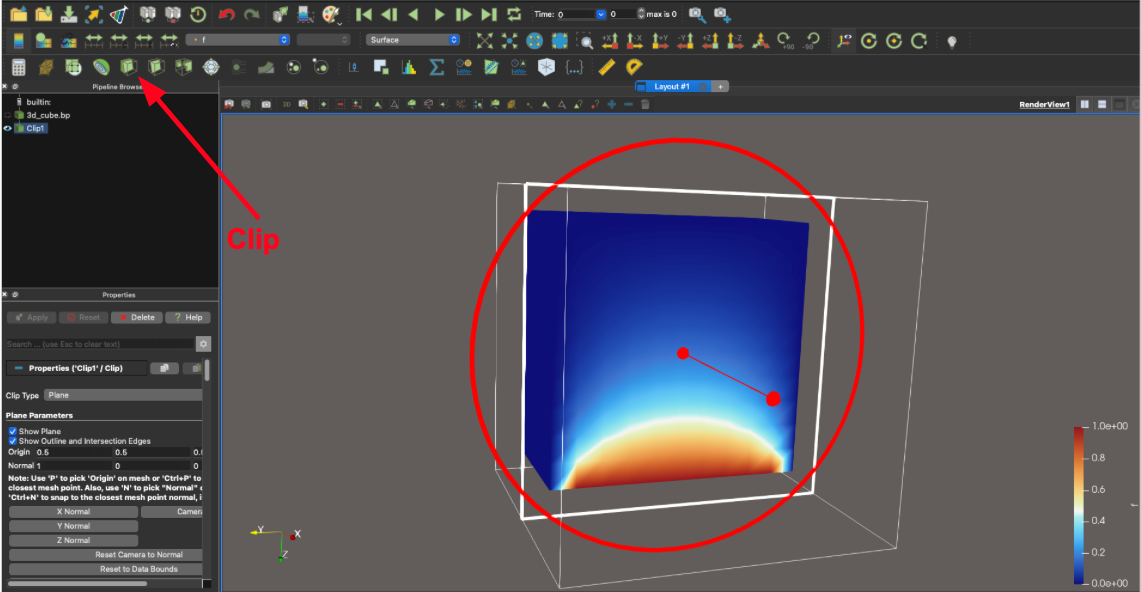
Let’s open our paraview/3d_cube.bp folder in ParaView and select the Clip option. Once you click Apply, this will produce a 3D volume that is partioned by a specified plane (in this case the YZ plane):

Similarly, we can view a 2D slice of our data by selecting our 3d_cube.bp file in the Pipeline Browser, then selecting Slice (shown below), and then selecting Apply:

Note

Be sure select your export file in the Pipeline Browser before clipping or slicing, otherwise your results will look empty.

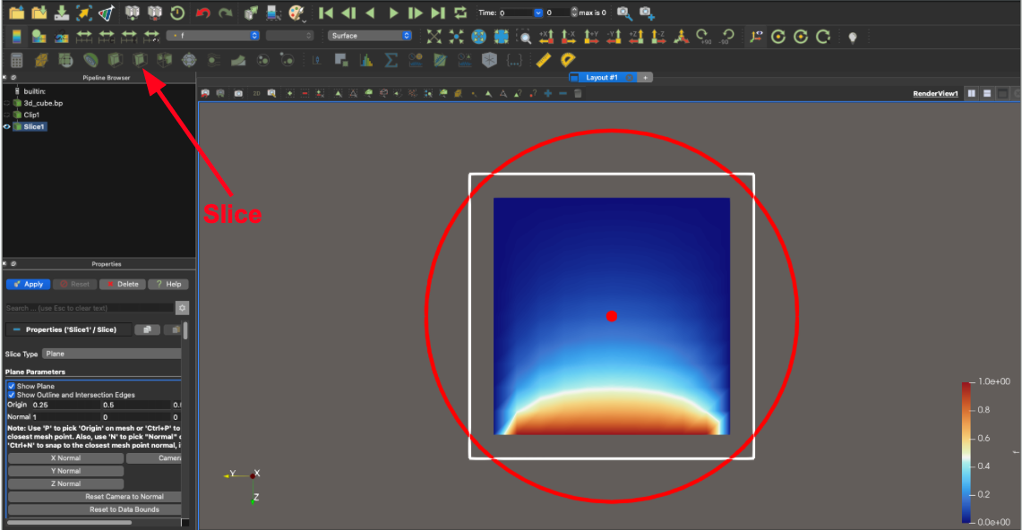
Tip

Users can select Show Plane box in the Plane Parameters window (usually on the left side of the screen) to show/hide the specified plane.