Chemical species#
Objectives
Learn how to define chemical species in FESTIM
Understand the concept of implicit species
Define explicit species#
In FESTIM, explicit species are species which concentrations are explicitly governed by a PDE in the governing equations.
For example, if consider the following problem:
In this case, the concentration of species 1 and 2 (namely \(c_1\) and \(c_2\)) are governed by a PDE. Species 1 and 2 are explicit species. In addition, they are mobile species since their governing equations exhibit a diffusive term.
In a FESTIM model, these species would be defined using the F.Species class:
Here’s another problem:
Here again, all species (1, 2, and 3) are explicitly accounted for in the governing equations. The three PDEs are coupled by a reaction. For more information on reactions, have a look at the Reactions tutorial.
This time Species 2 and 3 are immobile (ie. their governing equation don’t have a diffusive term).
The species would therefore be defined as:
Implicit species#
In some cases where we don’t want to explicitly define some species. Consider the following problem:
If we express \(c_2\) as:
And if we assume that \(n\) is known, then governing equations can therefore be written as:
Species 2 is, in this case, an implicit species. That is because its concentration can be directly expressed form other concentrations (here, \(n\) and \(c_3\)).
In this case, \(n\) can be any function of space and time. For example, \(n=2 x + y + 20 \ t\):
def n_fun(x, t):
    return 2 * x[0] + x[1] + 20 * t

species_2 = F.ImplicitSpecies(name="Species 2", n=n_fun, others=[species_3])
or in a more compact form:
species_2 = F.ImplicitSpecies(
    name="Species 2",
    n=lambda x, t: 2 * x[0] + x[1] + 20 * t,
    others=[species_3],
)
Using implicit species is useful for reducing the number of degrees of freedom in a problem.
Warning
ImplicitSpecies isn’t suitable for mobile species. That’s because their concentration cannot be expressed from other concentrations.
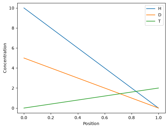
Complete example#
We consider the following problem on a 1D domain:
For simplicity, we assume that all three species have the same diffusivity.
Fixed concentration boundary conditions are set on both surfaces.
import festim as F
import numpy as np

my_model = F.HydrogenTransportProblem()

protium = F.Species("H")
deuterium = F.Species("D")
tritium = F.Species("T")
my_model.species = [protium, deuterium, tritium]

my_model.mesh = F.Mesh1D(np.linspace(0, 1, 100))

left_surf = F.SurfaceSubdomain1D(id=1, x=0)
right_surf = F.SurfaceSubdomain1D(id=2, x=1)

# assumes the same diffusivity for all species
material = F.Material(D_0=1, E_D=0)

vol = F.VolumeSubdomain1D(id=1, borders=[0, 1], material=material)

my_model.subdomains = [vol, left_surf, right_surf]

my_model.boundary_conditions = [
    # Protium BCs
    F.FixedConcentrationBC(left_surf, value=10, species=protium),
    F.FixedConcentrationBC(right_surf, value=0, species=protium),
    # Deuterium BCs
    F.FixedConcentrationBC(left_surf, value=5, species=deuterium),
    F.FixedConcentrationBC(right_surf, value=0, species=deuterium),
    # Tritium BCs
    F.FixedConcentrationBC(left_surf, value=0, species=tritium),
    F.FixedConcentrationBC(right_surf, value=2, species=tritium),
]

my_model.temperature = 300

my_model.settings = F.Settings(atol=1e-10, rtol=1e-10, final_time=100)

my_model.settings.stepsize = F.Stepsize(1)
my_model.initialise()
my_model.run()