

Coordinate systems#
Added in version 2.0: Cylindrical and spherical coordinate systems were introduced in FESTIM 2.0.
By default, FESTIM meshes use cartesian coordinates. For problems with cylindrical or spherical symmetry — such as a tube, a pipe wall, or a spherical pebble — it is much cheaper to solve a 1D problem in the radial direction than to build a full 2D or 3D mesh. FESTIM supports this through the coordinate_system argument of F.Mesh and F.Mesh1D.
Objectives:
Understand how the coordinate system affects the governing equations
Solve a radial diffusion problem in cylindrical and spherical coordinates
Why the coordinate system matters#
The steady-state diffusion equation \(\nabla \cdot (D \nabla c) = 0\) takes a different form depending on the coordinate system. For a purely radial problem:
Internally, FESTIM accounts for this by using the appropriate integration measure in the variational formulation (\(dr\), \(r\,dr\), and \(r^2\,dr\) respectively). As a result, the concentration profile between two fixed-concentration surfaces is linear in cartesian coordinates, logarithmic in cylindrical coordinates, and follows a \(1/r\) law in spherical coordinates.
Setting the coordinate system#
To use a non-cartesian coordinate system, simply pass coordinate_system when creating the mesh. Here the mesh coordinate represents the radius \(r\):
import numpy as np
import festim as F

mesh = F.Mesh1D(np.linspace(1, 2, 200), coordinate_system="cylindrical")
Note
The available coordinate systems are "cartesian" (default), "cylindrical", and "spherical". For a Mesh built from a dolfinx mesh, pass the same argument: F.Mesh(my_dolfinx_mesh, coordinate_system="cylindrical").
Example: radial diffusion#
Let us solve a steady-state radial diffusion problem between an inner radius \(r=1\) (where \(c=1\)) and an outer radius \(r=2\) (where \(c=0\)), and compare the three coordinate systems. We wrap the model in a function so we can run it for each system:
def solve(coordinate_system):
    my_model = F.HydrogenTransportProblem()
    my_model.mesh = F.Mesh1D(
        np.linspace(1, 2, 200), coordinate_system=coordinate_system
    )

    material = F.Material(D_0=1, E_D=0)
    vol = F.VolumeSubdomain1D(id=1, borders=[1, 2], material=material)
    inner = F.SurfaceSubdomain1D(id=1, x=1)
    outer = F.SurfaceSubdomain1D(id=2, x=2)

    H = F.Species("H")
    my_model.subdomains = [vol, inner, outer]
    my_model.species = [H]
    my_model.boundary_conditions = [
        F.FixedConcentrationBC(inner, value=1, species=H),
        F.FixedConcentrationBC(outer, value=0, species=H),
    ]
    my_model.temperature = 400
    my_model.settings = F.Settings(atol=1e-10, rtol=1e-10, transient=False)

    my_model.initialise()
    my_model.run()

    r = H.post_processing_solution.function_space.mesh.geometry.x[:, 0]
    c = H.post_processing_solution.x.array
    order = np.argsort(r)
    return r[order], c[order]
We now plot the concentration profile for each coordinate system, together with the analytical solutions:
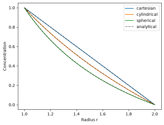
The FESTIM solutions (solid lines) match the analytical profiles (dashed) for all three coordinate systems, confirming that the geometry is correctly taken into account.
Warning
Derived quantities (e.g. SurfaceFlux, TotalVolume) are currently only implemented for cartesian coordinates. See this open issue for progress on non-cartesian derived quantities.