Hydrogen transport: basic

This section discusses how to implement basic boundary conditions (BCs) for hydrogen transport problems. Boundary conditions are essential to FESTIM simulations, as they describe the mathematical problem at the boundaries of the simulated domain. Read more about BCs here.

Objectives:

• Implement fixed concentration boundary conditions

• Implement particle flux boundary conditions

Imposing fixed concentration boundary conditions

Users can prescribe a fixed concentration on a boundary using FixedConcentrationBC, which can depend on temperature, time, and space.

Let us consider a 2D, steady-state, single-species example with the following space-dependent boundary conditions:

\[ \text{Top:} \quad c = 2x + y \]

\[ \text{Right:} \quad c = y^2 + 1 \]

Show code cell source

Hide code cell source

import festim as F
import numpy as np
from dolfinx.mesh import create_unit_square
from mpi4py import MPI

my_model = F.HydrogenTransportProblem()
my_model.mesh = F.Mesh(create_unit_square(MPI.COMM_WORLD, 10, 10))
H = F.Species("H")
my_model.species = [H]
mat = F.Material(D_0=1e-3, E_D=0)
my_model.material = mat
my_model.temperature = 400
my_model.settings = F.Settings(atol=1e-8, rtol=1e-8, transient=False)

/home/docs/checkouts/readthedocs.org/user_builds/festim-workshop/conda/latest/lib/python3.12/site-packages/festim/coupled_heat_hydrogen_problem.py:1: TqdmExperimentalWarning: Using `tqdm.autonotebook.tqdm` in notebook mode. Use `tqdm.tqdm` instead to force console mode (e.g. in jupyter console)
  import tqdm.autonotebook

Now, let’s create the boundaries to assign the BCs:

top_subdomain = F.SurfaceSubdomain(id=1, locator=lambda x: np.isclose(x[1], 1))
right_subdomain = F.SurfaceSubdomain(id=2, locator=lambda x: np.isclose(x[0], 1))
left_subdomain = F.SurfaceSubdomain(id=3, locator=lambda x: np.isclose(x[0], 0))
bottom_subdomain = F.SurfaceSubdomain(id=4, locator=lambda x: np.isclose(x[1], 0))
vol = F.VolumeSubdomain(id=5, material=mat)

my_model.subdomains = [top_subdomain, right_subdomain, left_subdomain, bottom_subdomain, vol]

We can define the top and right boundary conditions using lambda functions:

top_bc_function = lambda x: 2.0 * x[0] + x[1]
right_bc_function = lambda x: x[1] ** 2 + 1.0

Note

x[0], x[1], x[2] correspond to the first, second, and third space coordinate ( (x, y, z) in cartesian space). See Adding time and temperature dependent boundary conditions to learn more.

To include these boundary conditions to our problem, we use FixedConcentrationBC. We must also specify which subdomain (boundary) each BC is applied to, as well as the corresponding species:

top_bc = F.FixedConcentrationBC(
    subdomain=top_subdomain,
    value=top_bc_function,
    species=H
)

right_bc = F.FixedConcentrationBC(
    subdomain=right_subdomain,
    value=right_bc_function,
    species=H
)

We can add these to our problem, we pass them into boundary_conditions as a list and then run the simulation:

my_model.boundary_conditions = [top_bc, right_bc]
my_model.initialise()
my_model.run()

Show code cell source

Hide code cell source

import pyvista
from dolfinx import plot

topology, cell_types, geometry = plot.vtk_mesh(H.post_processing_solution.function_space)
grid = pyvista.UnstructuredGrid(topology, cell_types, geometry)
grid.point_data["c"] = H.post_processing_solution.x.array
grid.set_active_scalars("c")

pyvista.set_jupyter_backend("html")

plotter = pyvista.Plotter()

plotter.add_mesh(grid)
plotter.view_xy()
contours = grid.contour(isosurfaces=5, scalars="c")
if not pyvista.OFF_SCREEN:
    plotter.show()
else:
    figure = plotter.screenshot("concentration.png")

2026-05-22 15:20:58.915 (   0.826s) [    77D4A13C6740]vtkXOpenGLRenderWindow.:1458  WARN| bad X server connection. DISPLAY=

Note

In this example, we did not define any boundary conditions for the left and bottom surfaces. If no BC is set on a boundary, it is assumed that the flux is null (symmetry boundary condition):

\[ \mathbf{J} \cdot \mathbf{n} = 0 \quad \text{on } \Gamma \]

Adding time and temperature dependent boundary conditions

Users can also impose concentration BCs that are dependent on space \(x\), time \(t\), and temperature \(T\), such as:

\[ c = 10 + x^2 + T(t+2) \]

To do so, we define a Python function:

def my_custom_value(x, t, T):
    return 10 + x[0]**2 + T *(t + 2)

boundary = F.SurfaceSubdomain(id=1)
my_bc = F.FixedConcentrationBC(subdomain=boundary, value=my_custom_value, species=H)

Tip

This custom function is equivalent to:

my_custom_value = lambda x, t, T: 10 + x[0]**2 + T *(t + 2)

Multi-species fixed concentration BC

Users may also want to add BCs for multiple species in their model.

For example, if we wanted to impose separate fixed concentrations for deuterium and hydrogen on a boundary, we need to define each species and then one BC for each:

import festim as F

H = F.Species("H")
D = F.Species("D")
boundary = F.SurfaceSubdomain(id=1)

top_H = F.FixedConcentrationBC(
    subdomain=boundary,
    value=5.0,
    species=H
)

top_D = F.FixedConcentrationBC(
    subdomain=boundary,
    value=10.0,
    species=D
)       

Imposing particle flux boundary conditions

Users can impose the particle flux at boundaries using ParticleFluxBC class. At minimum, this BC requires a boundary, value, and species to be added:

import festim as F

boundary = F.SurfaceSubdomain(id=1)
H = F.Species(name="H")

my_flux_bc = F.ParticleFluxBC(subdomain=boundary, value=2, species=H)

To use this BC to your problem, simply add it to boundary_conditions attribute of your problem:

my_model = F.HydrogenTransportProblem()
my_model.boundary_conditions = [my_flux_bc]

Species-dependent fluxes

Similar to the concentration, the flux can be dependent on space, time and temperature. But for particle fluxes, the values can also be dependent on a species’ concentration.

For example, let’s define a hydrogen flux J that depends on the hydrogen concentration c and time t:

\[ J(c,t) = 10t^2 + 2c \]

import festim as F

my_model = F.HydrogenTransportProblem()
boundary = F.SurfaceSubdomain(id=1)
H = F.Species(name="H")

J = lambda t, c: 10*t**2 + 2*c

Note

A flux boundary condition dependent on the actual solution is called a Robin boundary condition.

To add this BC, we need to create a dictionary that maps the concentration variable c in our custom function to our species H:

mapping_dict = {"c": H}

Now, we add our ParticleFluxBC, also utilizing the species_dependent_value argument:

my_flux_bc = F.ParticleFluxBC(
    subdomain=boundary,
    value=J,
    species=H,
    species_dependent_value=mapping_dict,
)

my_model.boundary_conditions = [my_flux_bc]

Multi-species flux boundary conditions

Users may also need to impose a flux boundary condition which depends on the concentrations of multiple species.

Consider the following 1D example with three species, \(\mathrm{A}\), \(\mathrm{B}\), and \(\mathrm{C}\). The boundary conditions include recombination fluxes \(\phi_{AB}\) and \(\phi_{ABC}\) that depend on the concentrations \(\mathrm{c}\) (on the right) and fixed concentrations (on the left):

\[ \text{Right (recombination flux):} \quad \phi_{AB} = -c_A c_B \]

\[ \text{Right (recombination flux):} \quad \phi_{ABC} = -10 c_A c_B c_C\]

\[ \text{Left (fixed concentration):} \quad c_A = c_B = c_C = 1 \]

First, let us define each species using Species:

import festim as F

my_model = F.HydrogenTransportProblem()

A = F.Species(name="A")
B = F.Species(name="B")
C = F.Species(name="C")

my_model.species = [A, B, C]

Now, we create the dictionary to be passed into species_dependent_value; this maps each argument in the custom flux function to the corresponding defined species:

species_dependent_value = {"c_A": A, "c_B": B, "c_C": C}

We also define our custom functions for the fluxes:

recombination_flux_AB = lambda c_A, c_B, c_C: -c_A*c_B
recombination_flux_ABC = lambda c_A, c_B, c_C: -10*c_A*c_B*c_C

Now, we create our 1D mesh and corresponding boundaries:

import numpy as np

my_model.mesh = F.Mesh1D(np.linspace(0, 1, 100))

D = 1e-2
mat = F.Material(
    D_0={A: 8*D, B: 7*D, C: D},
    E_D={A: 0.01, B: 0.01, C: 0.01},
)

bulk = F.VolumeSubdomain1D(id=1, borders=[0, 1], material=mat)
left = F.SurfaceSubdomain1D(id=1, x=0)
right = F.SurfaceSubdomain1D(id=2, x=1)
my_model.subdomains = [bulk, left, right]

Note

The diffusivity pre-factor D_0 and activation energy E_D must be defined for each species in Material. Learn more about defining multi-species material properties here. Here we choose arbitrarily different diffusivity coefficients to see transport between species.

Let’s assign boundary conditions (recombination on the right, fixed concentration on the left). The boundary condition ParticleFluxBC must be added for each species:

my_model.boundary_conditions = [
    F.ParticleFluxBC(
        subdomain=right,
        value=recombination_flux_AB,
        species=A,
        species_dependent_value=species_dependent_value,
    ),
    F.ParticleFluxBC(
        subdomain=right,
        value=recombination_flux_AB,
        species=B,
        species_dependent_value=species_dependent_value,
    ),
    F.ParticleFluxBC(
        subdomain=right,
        value=recombination_flux_ABC,
        species=A,
        species_dependent_value=species_dependent_value,
    ),
    F.ParticleFluxBC(
        subdomain=right,
        value=recombination_flux_ABC,
        species=B,
        species_dependent_value=species_dependent_value,
    ),
    F.ParticleFluxBC(
        subdomain=right,
        value=recombination_flux_ABC,
        species=C,
        species_dependent_value=species_dependent_value,
    ),
    F.FixedConcentrationBC(subdomain=left,value=1,species=A),
    F.FixedConcentrationBC(subdomain=left,value=1,species=B),
    F.FixedConcentrationBC(subdomain=left,value=1,species=C),     
]

We can export the flux for each species on the right using SurfaceFlux (see post-processing derived values to learn more about exporting fluxes):

right_flux_A = F.SurfaceFlux(field=A,surface=right)
right_flux_B = F.SurfaceFlux(field=B,surface=right)
right_flux_C = F.SurfaceFlux(field=C,surface=right)

my_model.exports = [
    right_flux_A,
    right_flux_B,
    right_flux_C,
]

Finally, let’s solve and plot the profile for each species:

Show code cell source

Hide code cell source

my_model.temperature = 300
my_model.settings = F.Settings(atol=1e-10, rtol=1e-10, transient=False)

my_model.initialise()
my_model.run()

import matplotlib.pyplot as plt

def plot_profile(species, **kwargs):
    c = species.post_processing_solution.x.array[:]
    x = species.post_processing_solution.function_space.mesh.geometry.x[:,0]
    return plt.plot(x, c, **kwargs)

for species in my_model.species:
    plot_profile(species, label=species.name)

plt.xlabel('Position')
plt.ylabel('Concentration')
plt.legend()
plt.show()

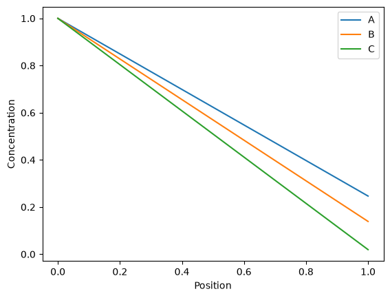
We see the higher recombination flux for \(\mathrm{ABC}\) decreases the concentration of \(\mathrm{C}\) throughout the material.