Hydrogen diffusion along grain boundaries#
This tutorial shows how to use FESTIM to simulate hydrogen diffusion in metal microstructures.
We’ll show how to generate a microstructure using Voronoi cells, mesh it with GMSH, and solve a transport problem with FESTIM.
Geometry#
Generating the microstructure#
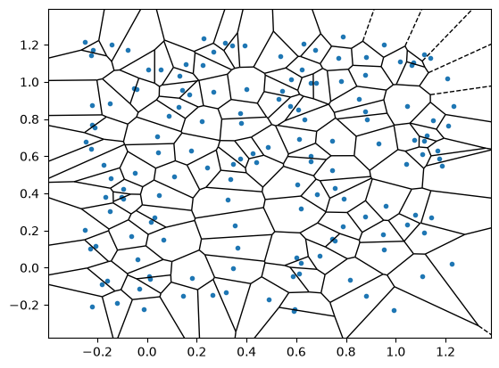
First, we use scipy to make a Voronoi diagram mimicking a microstructure.
import numpy as np
from scipy.spatial import Voronoi, voronoi_plot_2d
import matplotlib.pyplot as plt
import gmsh


np.random.seed(1)

# N random seeds in [0,size]x[0,size]
size = 1.5
N_seeds = 150
points = np.random.rand(N_seeds, 2) * size

# centre everything on 0.5, 0.5
points -= size / 2
points += 0.5

vor = Voronoi(points)

voronoi_plot_2d(vor, show_vertices=False, show_points=True)
plt.show()
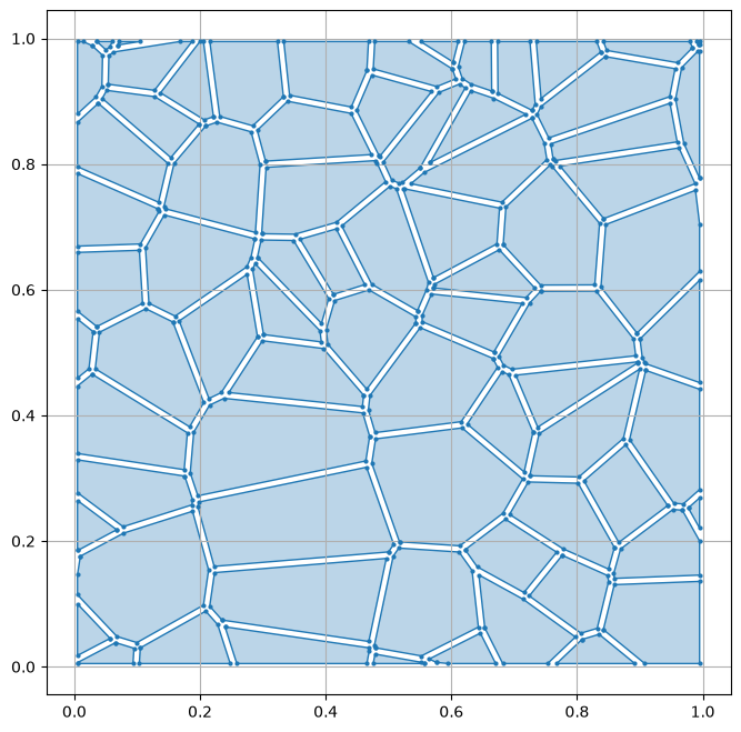
Now that we have vertices for each Voronoi cell, we can use shapely to turn them into shapely.Polygon objects for easy manipulation.
We then shrink the Voronoi cells to make grain boundaries appear. Note that the grain boundary thickness is arbitrary here.
from shapely.geometry import Polygon
from shapely import difference, union_all
from shapely.plotting import plot_polygon, plot_points

gap = 0.01  # thickness of grain boundary

grains = []
for region_idx in vor.point_region:
    region = vor.regions[region_idx]
    if -1 in region or len(region) == 0:
        continue  # skip infinite regions
    poly = Polygon([vor.vertices[i] for i in region])
    poly = poly.intersection(
        Polygon([(0, 0), (1, 0), (1, 1), (0, 1)])
    )  # clip to domain
    if not poly.is_empty:
        grains.append(poly.buffer(-gap / 2))  # shrink each grain inward

print("Number of grains:", len(grains))

plt.figure(figsize=(8, 8))
# plot grains
for polygon in grains:
    plot_polygon(polygon=polygon, add_points=False)
    plot_points(polygon, markersize=2, color="tab:blue")
plt.show()
Number of grains: 79
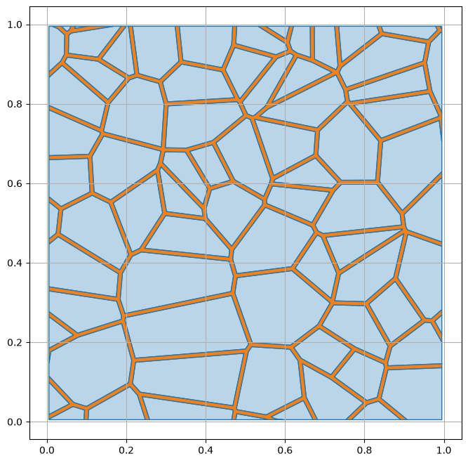
We can make a new Polygon for our grain boundaries by subtracting all the grains from a square polygon.
# Grain boundary = everything not covered by grains
eps = gap / 2
domain = Polygon(
    [(0 + eps, 0 + eps), (1 - eps, 0 + eps), (1 - eps, 1 - eps), (0 + eps, 1 - eps)]
)
grain_union = union_all(grains)
grain_boundaries = difference(domain, grain_union)

plt.figure(figsize=(8, 8))
for polygon in grains:
    plot_polygon(polygon=polygon, add_points=False)
plot_polygon(polygon=grain_boundaries, facecolor="tab:orange", add_points=False)
plt.show()
Mesh with GMSH#
We can now pass this geometry to GMSH for meshing. We tag the grains, grain boundaries, and the left and right surfaces as different subdomains.
gmsh.initialize()
gmsh.model.add("voronoi")

lc = 0.01  # mesh size


def add_polygon_occ(poly):
    """Add polygon using OpenCASCADE kernel for better Boolean operations"""
    if poly.is_empty:
        return []

    # Handle MultiPolygon recursively
    if poly.geom_type == "MultiPolygon":
        surfaces = []
        for p in poly.geoms:
            surfaces.extend(add_polygon_occ(p))
        return surfaces

    # Ensure polygon is valid
    poly = poly.buffer(0)
    if not poly.is_valid:
        return []

    # exterior coords
    coords = list(poly.exterior.coords)[:-1]  # remove duplicate last point
    if len(coords) < 3:
        return []

    # Create wire from points using OCC
    points = []
    for x, y in coords:
        points.append(gmsh.model.occ.addPoint(x, y, 0))

    # Create lines connecting the points
    lines = []
    for i in range(len(points)):
        next_i = (i + 1) % len(points)
        lines.append(gmsh.model.occ.addLine(points[i], points[next_i]))

    # Create curve loop and surface
    wire = gmsh.model.occ.addWire(lines)

    # Handle holes if any
    holes = []
    if len(poly.interiors) > 0:
        for interior in poly.interiors:
            int_coords = list(interior.coords)[:-1]
            if len(int_coords) < 3:
                continue

            # Create hole wire
            hole_points = []
            for x, y in int_coords:
                hole_points.append(gmsh.model.occ.addPoint(x, y, 0))

            hole_lines = []
            for i in range(len(hole_points)):
                next_i = (i + 1) % len(hole_points)
                hole_lines.append(
                    gmsh.model.occ.addLine(hole_points[i], hole_points[next_i])
                )

            hole_wire = gmsh.model.occ.addWire(hole_lines)
            holes.append(hole_wire)

    # Create surface
    if holes:
        surface = gmsh.model.occ.addPlaneSurface([wire] + holes)
    else:
        surface = gmsh.model.occ.addPlaneSurface([wire])

    return [surface]


# Add grains using OCC kernel
grain_surfaces = []
for i, poly in enumerate(grains):
    grain_surfaces.extend(add_polygon_occ(poly))

gb_surfaces = []
if not grain_boundaries.is_empty:
    gb_surfaces.extend(add_polygon_occ(grain_boundaries))

# Synchronize OCC before fragmentation
gmsh.model.occ.synchronize()

# Fragment all surfaces together
gmsh.model.occ.fragment([(2, tag) for tag in grain_surfaces], [(2, gb_surfaces[0])])
gmsh.model.occ.synchronize()

# Create physical groups with all fragmented surfaces

gmsh.model.addPhysicalGroup(2, grain_surfaces, 1, name="grains")
gmsh.model.addPhysicalGroup(2, gb_surfaces, 2, name="grain_boundaries")

# Set mesh size for all points
gmsh.option.setNumber("Mesh.MeshSizeMax", lc)
gmsh.option.setNumber("Mesh.MeshSizeMin", lc)

# find lines on the boundaries
# Get all line entities (dimension = 1)
lines = gmsh.model.getEntities(1)

# List to store the tags of the lines on the boundaries
lines_on_left = []
lines_on_right = []

for line_tag_pair in lines:
    dim = line_tag_pair[0]  # Dimension of the entity (1 for lines)
    tag = line_tag_pair[1]  # Tag of the entity

    # Get the bounding points (dimension = 0) for the current line
    bounding_points = gmsh.model.getBoundary([line_tag_pair])

    # Get the coordinates for each bounding point
    point_coords = []
    for point_tag_pair in bounding_points:
        coords = gmsh.model.getValue(point_tag_pair[0], point_tag_pair[1], [])
        point_coords.append(coords)

    # Check if both bounding points are on the left boundary (x ≈ eps)
    is_on_left = True
    for coords in point_coords:
        x_coord = coords[0]
        if abs(x_coord - eps) > 1e-9:
            is_on_left = False
            break

    # Check if both bounding points are on the right boundary (x ≈ 1-eps)
    is_on_right = True
    for coords in point_coords:
        x_coord = coords[0]
        if abs(x_coord - (1 - eps)) > 1e-9:
            is_on_right = False
            break

    if is_on_left:
        lines_on_left.append(tag)
    if is_on_right:
        lines_on_right.append(tag)

print("Lines on left boundary:", lines_on_left)
print("Lines on right boundary:", lines_on_right)

if lines_on_left:
    gmsh.model.addPhysicalGroup(1, lines_on_left, name="left_boundary")
if lines_on_right:
    gmsh.model.addPhysicalGroup(1, lines_on_right, name="right_boundary")

gmsh.model.mesh.generate(2)
# gmsh.fltk.run()
gmsh.write("voronoi_grains.msh")

gmsh.finalize()
FESTIM model#
We can now define our hydrogen transport problem.
where \(D=D_\mathrm{GB}\) and \(D=D_\mathrm{grain}\) in the grain boundary and grain, respectively.
Boundary conditions:
\( c = 0 \) on the left surface
\( c = 1 \) on the right surface
Interface condition:
We assume continuity of concentration at the GB/grain interfaces.
Simulation time: \(t_f = 1.5\)
Convert mesh to dolfinx#
from dolfinx.io import gmsh as gmshio
from mpi4py import MPI


model_rank = 0
mesh_data = gmshio.read_from_msh(
    "voronoi_grains.msh", MPI.COMM_WORLD, 0, gdim=2
)
mesh = mesh_data.mesh
assert mesh_data.facet_tags is not None
facet_tags = mesh_data.facet_tags
facet_tags.name = "Facet markers"

assert mesh_data.cell_tags is not None
cell_tags = mesh_data.cell_tags
cell_tags.name = "Cell markers"
Info    : Reading 'voronoi_grains.msh'...
Info    : 927 entities
Info    : 13269 nodes
Info    : 26318 elements
Info    : Done reading 'voronoi_grains.msh'
2026-07-15 17:27:49.275 ( 3.885s) [ 7FE8BA8CE440]vtkXOpenGLRenderWindow.:1458 WARN| bad X server connection. DISPLAY=
Case 1: GBs are more diffusive#
In this first case, \(D_\mathrm{GB}= 1000 \ D_\mathrm{grain}\)
import festim as F

grain_mat = F.Material(D_0=0.001, E_D=0)
gb_mat = F.Material(D_0=1, E_D=0)


grain_vol = F.VolumeSubdomain(id=1, material=grain_mat)
gb_vol = F.VolumeSubdomain(id=2, material=gb_mat)

left_surf = F.SurfaceSubdomain(id=3)
right_surf = F.SurfaceSubdomain(id=4)

my_model = F.HydrogenTransportProblem()

my_model.mesh = F.Mesh(mesh)

# we need to pass the meshtags to the model directly
my_model.facet_meshtags = facet_tags
my_model.volume_meshtags = cell_tags

my_model.subdomains = [left_surf, right_surf, grain_vol, gb_vol]

H = F.Species("H")
my_model.species = [H]

my_model.temperature = 400

my_model.boundary_conditions = [
    F.FixedConcentrationBC(subdomain=left_surf, value=0, species=H),
    F.FixedConcentrationBC(subdomain=right_surf, value=1, species=H),
]

my_model.settings = F.Settings(atol=1e-10, rtol=1e-20, final_time=1.5)
my_model.settings.stepsize = 0.01

my_model.exports = [F.VTXSpeciesExport(filename="out.bp", field=H)]

my_model.initialise()
my_model.run()
At the end of the simulation, we can see on the concentration field the preferential diffusion along the grain boundaries!
Case 2: GBs are less diffusive#
We can also look at the opposite case with grain boundaries less diffusive the the grain themselves.
gb_mat.D_0 = 0.1
grain_mat.D_0 = 1

my_model.initialise()
my_model.run()