Transient problem

Transient problem#

Now that we’ve solve a steady state problem, we’re going to step it up by solving a transient problem. We’ll use the same geometry and similar parameters.

We’ll also set the same boundary conditions with the difference that the value of one of the conditions will change with time. The complete mathematical problem is:

(23)#\[\begin{align} \frac{\partial c_m}{\partial t} &= \nabla \cdot (D \nabla c_m) - R \quad \text{on } \Omega\\ \frac{\partial c_t}{\partial t} &= + R \quad \text{on } \Omega\\ R &= k c_m (n - c_t) - p \ c_t \\ c_m &= \begin{cases} 1 \quad \text{for } t < 5 \\ 0 \quad \text{otherwise} \end{cases} \quad \text{on } \Gamma_\mathrm{inlet} \\ c_m &= 0\quad \text{on } \Gamma_\mathrm{outlet} \end{align}\]

Setting up#

import dolfinx
import numpy as np
import ufl
from dolfinx.fem.petsc import NonlinearProblem
from petsc4py import PETSc
from mpi4py import MPI
from dolfinx import mesh
from dolfinx import fem
import basix
from scifem import assemble_scalar

nx = ny = 20

domain = mesh.create_unit_square(MPI.COMM_WORLD, nx, ny, mesh.CellType.quadrilateral)

# we create a mixed element with two components, both continuous galerkin degree 1
cg_element = basix.ufl.element("Lagrange", domain.basix_cell(), degree=1)

mixed_element = basix.ufl.mixed_element([cg_element, cg_element])

# then we make a functionspace from the mixed element
V = fem.functionspace(domain, mixed_element)

# we create a "main" function u which is a vector of the two components
u = fem.Function(V)

# and a u_n function for the previous time step
u_n = fem.Function(V)

# to use the components in variational forms, we use ufl.split
# the first will be the mobile concentration cm, the second the trapped concentration ct
cm, ct = ufl.split(u)
cm_n, ct_n = ufl.split(u_n)

# we create test functions for both components
v_cm, v_ct = ufl.TestFunctions(V)

We use the same boudary conditions as the steady state case, with the exception that we will modify the value of c_inlet at \(t=5\) to highlight transient effects.

def inlet(x):
    return np.logical_and(np.isclose(x[0], 0), x[1] <= 0.5)

def outlet(x):
    return np.logical_and(np.isclose(x[0], 1), x[1] >= 0.5)

V0, submap = V.sub(0).collapse()

# the trick here was to pass both the subspace and the collapsed space to locate_dofs_geometrical
# in FESTIM we don't need this since we use meshtags for everything
# https://fenicsproject.discourse.group/t/dolfinx-dirichlet-bcs-for-mixed-function-spaces/7844/2

dofs_outlet = fem.locate_dofs_geometrical((V.sub(0), V0), outlet)
dofs_inlet = fem.locate_dofs_geometrical((V.sub(0), V0), inlet)

c_inlet = fem.Constant(domain, 1.0)
c_outlet = fem.Constant(domain, 0.0)

bc_outlet = fem.dirichletbc(c_outlet, dofs_outlet[0], V.sub(0))
bc_inlet = fem.dirichletbc(c_inlet, dofs_inlet[0], V.sub(0))

The variational formulation is extremely similar, we just add a transient term using a first order backwards Euler time-stepping scheme.

# Problem parameters
k = 0.2  # trapping rate
p = 0.01  # detrapping rate
n = 0.5  # total trapping sites
D = 0.1 # diffusion coefficient

dt = dolfinx.fem.Constant(domain, 1.0)


# NOTE everything is bundled in one variational form F
# the difference between the different equations is made with the test functions v_cm and v_ct
F_mobile_transient = (cm - cm_n)/dt* v_cm * ufl.dx
F_trapped_transient = (ct - ct_n)/dt * v_ct * ufl.dx


trapping = k * cm * (n - ct)
detrapping = p * ct

F_mobile = (
    D*ufl.dot(ufl.grad(cm), ufl.grad(v_cm)) * ufl.dx
    + trapping * v_cm * ufl.dx
    - detrapping * v_cm * ufl.dx
)
F_trapped = -trapping * v_ct * ufl.dx + detrapping * v_ct * ufl.dx

F = F_mobile_transient + F_trapped_transient + F_mobile + F_trapped

We set up the nonlinear solver in the exact same way:

# taken from https://github.com/FEniCS/dolfinx/blob/5fcb988c5b0f46b8f9183bc844d8f533a2130d6a/python/demo/demo_cahn-hilliard.py#L279C1-L286C28
use_superlu = PETSc.IntType == np.int64  # or PETSc.ScalarType == np.complex64
sys = PETSc.Sys()  # type: ignore
if sys.hasExternalPackage("mumps") and not use_superlu:
    linear_solver = "mumps"
elif sys.hasExternalPackage("superlu_dist"):
    linear_solver = "superlu_dist"
else:
    linear_solver = "petsc"

petsc_options = {
    "snes_type": "newtonls",
    "snes_linesearch_type": "none",
    "snes_stol": np.sqrt(np.finfo(dolfinx.default_real_type).eps) * 1e-2,
    "snes_atol": 1e-10,
    "snes_rtol": 1e-10,
    "snes_max_it": 100,
    "snes_divergence_tolerance": "PETSC_UNLIMITED",
    "ksp_type": "preonly",
    "pc_type": "lu",
    "pc_factor_mat_solver_type": linear_solver,
    # "snes_monitor": None,
}

problem = NonlinearProblem(
    F,
    u,
    bcs=[bc_outlet, bc_inlet],
    petsc_options=petsc_options,
    petsc_options_prefix="poisson_transient",
)

Let’s prepare a pyvista animation:

import pyvista
import matplotlib as mpl
from dolfinx import plot

c_m_post = u.split()[0].collapse()
c_t_post = u.split()[1].collapse()

grid_c_m = pyvista.UnstructuredGrid(*plot.vtk_mesh(c_m_post.function_space))
grid_c_t = pyvista.UnstructuredGrid(*plot.vtk_mesh(c_t_post.function_space))

grid_c_m.point_data["c_m"] = c_m_post.x.array
grid_c_t.point_data["c_t"] = c_t_post.x.array

viridis = mpl.colormaps.get_cmap("viridis").resampled(50)
sargs = dict(
    title_font_size=25,
    label_font_size=20,
    fmt="%.2e",
    color="black",
    position_x=0.1,
    position_y=0.8,
    width=0.8,
    height=0.1,
)

plotter = pyvista.Plotter(shape=(1, 2))
plotter.open_gif("transient.gif", fps=7)

plotter.subplot(0, 0)
plotter.view_xy(bounds=[0, 1, 0, 1, 0, 0])
_ = plotter.add_mesh(
    grid_c_m,
    show_edges=False,
    lighting=False,
    cmap=viridis,
    scalar_bar_args=sargs,
    clim=[0, 1],
)

plotter.subplot(0, 1)
plotter.view_xy(bounds=[0, 1, 0, 1, 0, 0])

_ = plotter.add_mesh(
    grid_c_t,
    show_edges=False,
    lighting=False,
    cmap=viridis,
    scalar_bar_args=sargs,
    clim=[0, n],
)

2026-05-22 15:22:54.504 (   0.580s) [    702006D21740]vtkXOpenGLRenderWindow.:1458  WARN| bad X server connection. DISPLAY=

Solving#

We make two empty lists for storing the inventory values:

inventories_cm = []
inventories_ct = []
times = []

dolfinx doesn’t “know” anything about time. We set the time stepping loop ourselves.

At each timestep we:

update t
solve the nonlinear problem
update the previous solution u_n
update the inlet boundary condition
perform the post processing tasks

t = 0.0
t_final = 30
n_it = 0

while t < t_final:
    t += dt.value
    n_it += 1
    times.append(t)

    # solve the problem with the current u_n as previous solution
    problem.solve()
    converged = problem.solver.getConvergedReason()
    num_iter = problem.solver.getIterationNumber()
    assert converged > 0, f"Solver did not converge, got {converged}."
    print(
        f"Time: {t:.2f} ({n_it=}). \n Solver converged after {num_iter} iterations with converged reason {converged}."
    )

    # update u_n with the current solution u
    u_n.x.array[:] = u.x.array[:]

    # update inlet value to show transient response
    c_inlet.value = 1.0 if t < 5 else 0.0

    # post processing
    c_m_post = u.split()[0].collapse()
    c_t_post = u.split()[1].collapse()

    # Update plot
    grid_c_m.point_data["c_m"][:] = c_m_post.x.array
    grid_c_t.point_data["c_t"][:] = c_t_post.x.array
    plotter.write_frame()

    # compute inventory
    inventories_cm.append(assemble_scalar(c_m_post * ufl.dx))
    inventories_ct.append(assemble_scalar(c_t_post * ufl.dx))

plotter.close()

Time: 1.00 (n_it=1). 
 Solver converged after 3 iterations with converged reason 2.
Time: 2.00 (n_it=2). 
 Solver converged after 3 iterations with converged reason 2.
Time: 3.00 (n_it=3). 
 Solver converged after 3 iterations with converged reason 2.

Time: 4.00 (n_it=4). 
 Solver converged after 3 iterations with converged reason 2.
Time: 5.00 (n_it=5). 
 Solver converged after 3 iterations with converged reason 2.
Time: 6.00 (n_it=6). 
 Solver converged after 3 iterations with converged reason 2.
Time: 7.00 (n_it=7). 
 Solver converged after 3 iterations with converged reason 2.
Time: 8.00 (n_it=8). 
 Solver converged after 2 iterations with converged reason 2.

Time: 9.00 (n_it=9). 
 Solver converged after 2 iterations with converged reason 2.
Time: 10.00 (n_it=10). 
 Solver converged after 2 iterations with converged reason 2.
Time: 11.00 (n_it=11). 
 Solver converged after 2 iterations with converged reason 2.
Time: 12.00 (n_it=12). 
 Solver converged after 2 iterations with converged reason 2.
Time: 13.00 (n_it=13). 
 Solver converged after 2 iterations with converged reason 2.

Time: 14.00 (n_it=14). 
 Solver converged after 2 iterations with converged reason 2.
Time: 15.00 (n_it=15). 
 Solver converged after 2 iterations with converged reason 2.
Time: 16.00 (n_it=16). 
 Solver converged after 2 iterations with converged reason 2.
Time: 17.00 (n_it=17). 
 Solver converged after 2 iterations with converged reason 2.

Time: 18.00 (n_it=18). 
 Solver converged after 2 iterations with converged reason 2.
Time: 19.00 (n_it=19). 
 Solver converged after 2 iterations with converged reason 2.
Time: 20.00 (n_it=20). 
 Solver converged after 2 iterations with converged reason 2.
Time: 21.00 (n_it=21). 
 Solver converged after 2 iterations with converged reason 2.

Time: 22.00 (n_it=22). 
 Solver converged after 2 iterations with converged reason 2.
Time: 23.00 (n_it=23). 
 Solver converged after 2 iterations with converged reason 2.
Time: 24.00 (n_it=24). 
 Solver converged after 2 iterations with converged reason 2.
Time: 25.00 (n_it=25). 
 Solver converged after 2 iterations with converged reason 2.

Time: 26.00 (n_it=26). 
 Solver converged after 2 iterations with converged reason 2.
Time: 27.00 (n_it=27). 
 Solver converged after 2 iterations with converged reason 2.
Time: 28.00 (n_it=28). 
 Solver converged after 2 iterations with converged reason 2.
Time: 29.00 (n_it=29). 
 Solver converged after 2 iterations with converged reason 2.

Time: 30.00 (n_it=30). 
 Solver converged after 2 iterations with converged reason 2.

gif

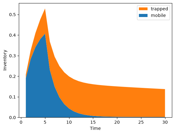
import matplotlib.pyplot as plt

plt.stackplot(times, inventories_cm, inventories_ct, labels=["mobile", "trapped"])
plt.ylabel("Inventory")
plt.xlabel("Time")
plt.legend(reverse=True)
plt.show()

../../_images/23b15a1815b59ffd8b3d27afe963c0d93d2080024246d889364febe43b5ccdd3.png

Transient problem

Contents

Transient problem#

Setting up#

Solving#