Advanced functionality#
This tutorial introduces more advanced ways of handling materials in FESTIM. A key addition in FESTIM 2.0 is the ability to perform multi-species simulations, which often requires assigning distinct material properties to each species (see documentation for more information). In some cases, users may also need to define custom material properties—for example, specifying a turbulence-dependent viscosity or user-defined diffusivity.
Objectives:
Assign different material properties to different species
Solve a problem with custom material properties (e.g., diffusivity)
Defining species-dependent material properties#
Consider the following 1D example that simulates the diffusion of protium, deuterium and tritium:
import festim as F
import numpy as np

my_model = F.HydrogenTransportProblem()

protium = F.Species("H")
deuterium = F.Species("D")
tritium = F.Species("T")
my_model.species = [protium, deuterium, tritium]

my_model.mesh = F.Mesh1D(np.linspace(0, 1, 100))

left_surf = F.SurfaceSubdomain1D(id=1, x=0)
right_surf = F.SurfaceSubdomain1D(id=2, x=1)
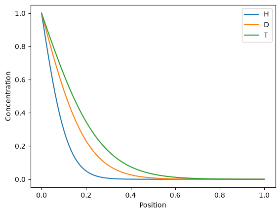
Here we define the different diffusivities (or rather the diffusivities’ pre-exponential factors) for each species.
Instead of passing a single value to the D_0 of Material, we pass a dictionary where the keys are the different Species objects and values are values of pre-exponential factors D_0 and activation energy E_D.
We define one domain called bulk and attach the material to it:
mat = F.Material(
    D_0={protium: 1.0e-3, deuterium: 3.0e-3, tritium: 5.0e-3},
    E_D={protium: 0.0, deuterium: 0.0, tritium: 0.0},
)

bulk = F.VolumeSubdomain1D(id=1, borders=[0, 1], material=mat)

my_model.subdomains = [bulk, left_surf, right_surf]
To illustrate how different species’ diffusion properties affect the simulation, we set the same boundary condition for each species (1 on the left boundary, 0 on the right). Now we can run the simulation and look at the concentration profile for each species:
# Boundary conditions
my_model.boundary_conditions = [
    F.FixedConcentrationBC(left_surf, value=1, species=protium),
    F.FixedConcentrationBC(right_surf, value=0, species=protium),
    F.FixedConcentrationBC(left_surf, value=1, species=deuterium),
    F.FixedConcentrationBC(right_surf, value=0, species=deuterium),
    F.FixedConcentrationBC(left_surf, value=1, species=tritium),
    F.FixedConcentrationBC(right_surf, value=0, species=tritium),
]

my_model.temperature = 300
my_model.settings = F.Settings(atol=1e-10, rtol=1e-10, final_time=5)

my_model.settings.stepsize = F.Stepsize(1)
my_model.initialise()
my_model.run()
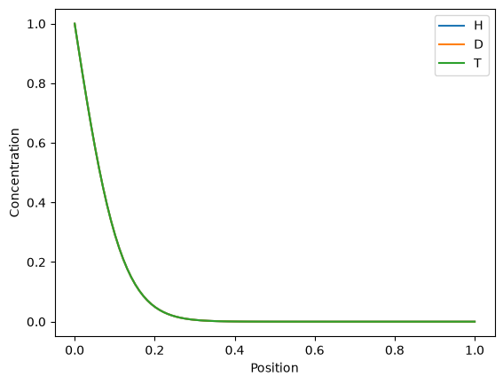
Compare this to the case where each species has the same diffusion properties:
mat.D_0 = {protium: 1.0e-3, deuterium: 1.0e-3, tritium: 1.0e-3}
my_model.initialise()
my_model.run()
Custom diffusion coefficient#
Some cases will require user-defined material properties (such as in bubbly flows or turbulence-assisted-diffusion).
In this 2D example, we show how to define a spatially-dependent diffusivity. Specifcally, we’ll look at a circular diffusivity profile: \( D = 0.1 + x^2 + y^2 \)
First, we need to define a 2D mesh:
import dolfinx
from dolfinx.mesh import create_unit_square
from mpi4py import MPI
import numpy as np
import festim as F
from basix.ufl import element
from dolfinx import plot
import pyvista

mesh_fenics = create_unit_square(MPI.COMM_WORLD, 20, 20)
my_model = F.HydrogenTransportProblem()
my_model.mesh = F.Mesh(mesh_fenics)
Users can define a spatially-dependent material property using fem.Function, which requires a function space (with the correct order) to be setup using fem.functionspace:
el = element("Lagrange", mesh_fenics.topology.cell_name(), 2)
V = dolfinx.fem.functionspace(my_model.mesh.mesh, el)

# Define diffusion coefficient as scalar field
diffusivity = dolfinx.fem.Function(V)
diffusivity.interpolate(lambda x: 0.1 + x[0]**2 + x[1]**2)
Here’s our diffusivity field:
2026-07-15 17:32:50.971 ( 0.570s) [ 7ACD722CD440]vtkXOpenGLRenderWindow.:1458 WARN| bad X server connection. DISPLAY=
Now we can add this property directly to a FESTIM Material:
my_mat = F.Material(D=diffusivity) # m²/s
Finally, let’s solve the problem and visualize the results:
# Species
H = F.Species("H")
my_model.species = [H]

# Subdomains
volume = F.VolumeSubdomain(id=1, material=my_mat)
top_surface = F.SurfaceSubdomain(id=2, locator=lambda x: np.isclose(x[1], 1.0))
bottom_surface = F.SurfaceSubdomain(id=3, locator=lambda x: np.isclose(x[1], 0.0))
my_model.subdomains = [volume, top_surface, bottom_surface]

# Temperature
my_model.temperature = 600  # K

# Boundary conditions
my_model.boundary_conditions = [
    F.FixedConcentrationBC(subdomain=top_surface, value=1.0, species=H),
    F.FixedConcentrationBC(subdomain=bottom_surface, value=0.0, species=H),
]

# Solver settings
my_model.settings = F.Settings(atol=1e-10, rtol=1e-10, transient=False)

# Run simulation
my_model.initialise()
my_model.run()