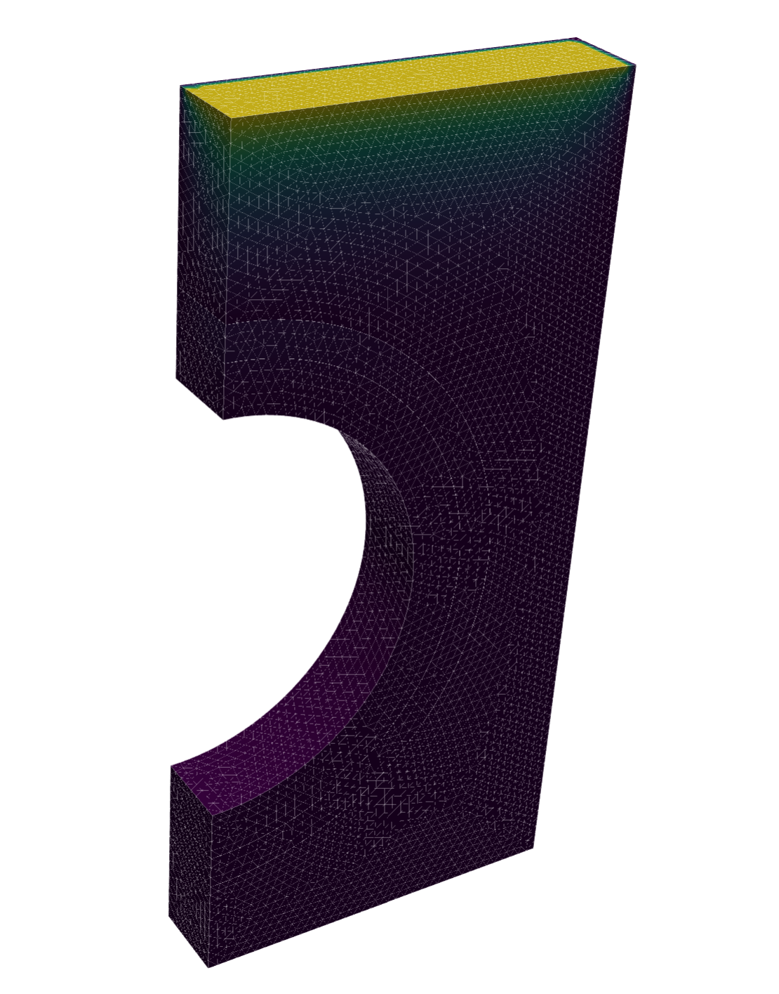
Monoblock#
In this application case we will simulate heat transfer and hydrogen transport in a 3D ITER-like monoblock made of three different materials (tungsten, cucrzr, and copper).
See also
Simulating tritium transport in plasma-facing components was one of the very first applications of FESTIM.
Mesh#
We start by reading a .med mesh file from SALOME and convert it to XDMF using meshio.
See also
Meshes for more details on meshing in FESTIM
correspondance_dict, cell_data_types = convert_med_to_xdmf(
"task08/mesh.med",
cell_file="task08/mesh_domains.xdmf",
facet_file="task08/mesh_boundaries.xdmf",
)
The correspondance_dict will be extremely useful to assign an id to each subdomain:
for index, label in correspondance_dict.items():
print(f"{index}: {label[0]}")
6: tungsten
7: copper
8: cucrzr
9: top_surface
10: coolant_surface
11: poloidal_tungsten
12: poloidal_copper
13: poloidal_cucrzr
14: toroidal
15: bottom
16: interface_tungsten_copper
17: interface_copper_cucrzr
The converted .xdmf files can then be imported in FESTIM using the MeshFromXDMF class:
import festim as F
mesh = F.MeshFromXDMF(
volume_file="task08/mesh_domains.xdmf", facet_file="task08/mesh_boundaries.xdmf"
)
mesh.mesh.geometry.x[:] *= 1e-3 # mm to m
# rotate to have z as the vertical axis
mesh.mesh.geometry.x[:, [0, 1, 2]] = mesh.mesh.geometry.x[:, [0, 2, 1]]
2026-07-15 17:30:18.753 ( 1.194s) [ 7130DE58C440]vtkXOpenGLRenderWindow.:1458 WARN| bad X server connection. DISPLAY=
Subdomains and materials#
We start by defining three materials for tungsten, copper, and CuCrZr
tungsten = F.Material(
D_0=4.1e-7,
E_D=0.39,
K_S_0=1.87e24,
E_K_S=1.04,
thermal_conductivity=100,
)
copper = F.Material(
D_0=6.6e-7,
E_D=0.387,
K_S_0=3.14e24,
E_K_S=0.572,
thermal_conductivity=350,
)
cucrzr = F.Material(
D_0=3.92e-7,
E_D=0.418,
K_S_0=4.28e23,
E_K_S=0.387,
thermal_conductivity=350,
)
Using the tags provided by correspondance_dict, we can create volume and surface subdomains and assign them materials:
tungsten_volume = F.VolumeSubdomain(id=6, material=tungsten)
copper_volume = F.VolumeSubdomain(id=7, material=copper)
cucrzr_volume = F.VolumeSubdomain(id=8, material=cucrzr)
top_surface = F.SurfaceSubdomain(id=9)
cooling_surface = F.SurfaceSubdomain(id=10)
poloidal_gap_w = F.SurfaceSubdomain(id=11)
poloidal_gap_cu = F.SurfaceSubdomain(id=12)
poloidal_gap_cucrzr = F.SurfaceSubdomain(id=13)
toroidal_gap = F.SurfaceSubdomain(id=14)
bottom = F.SurfaceSubdomain(id=15)
all_subdomains = [
tungsten_volume,
copper_volume,
cucrzr_volume,
top_surface,
cooling_surface,
poloidal_gap_cu,
poloidal_gap_w,
poloidal_gap_cucrzr,
toroidal_gap,
bottom,
]
Solving the heat transfer problem#
heat_transfer_problem = F.HeatTransferProblem()
# Mesh and subdomains
heat_transfer_problem.subdomains = all_subdomains
heat_transfer_problem.mesh = mesh
# Boundary conditions
heat_flux_top = F.HeatFluxBC(subdomain=top_surface, value=10e6)
h_convective = 7e04 # W/m^2/K
T_coolant = 323 # K
convective_flux_coolant = F.HeatFluxBC(
subdomain=cooling_surface, value=lambda T: h_convective * (T_coolant - T)
)
heat_transfer_problem.boundary_conditions = [heat_flux_top, convective_flux_coolant]
# Exports
heat_transfer_problem.exports = [F.VTXTemperatureExport("out.bp")]
# Settings
heat_transfer_problem.settings = F.Settings(
atol=1e-10,
rtol=1e-10,
transient=False,
)
# Run
heat_transfer_problem.initialise()
heat_transfer_problem.run()
Solving the tritium transport problem#
my_model = F.HydrogenTransportProblemDiscontinuous()
my_model.method_interface = "penalty"
my_model.subdomains = all_subdomains
H = F.Species("H", subdomains=my_model.volume_subdomains)
my_model.species = [H]
my_model.mesh = mesh
my_model.surface_to_volume = {
top_surface: tungsten_volume,
cooling_surface: cucrzr_volume,
poloidal_gap_w: tungsten_volume,
poloidal_gap_cu: copper_volume,
poloidal_gap_cucrzr: cucrzr_volume,
toroidal_gap: tungsten_volume,
bottom: tungsten_volume,
}
penalty_term = 1e20
my_model.interfaces = [
F.Interface(
id=16, subdomains=(tungsten_volume, copper_volume), penalty_term=penalty_term
),
F.Interface(
id=17, subdomains=(copper_volume, cucrzr_volume), penalty_term=penalty_term
),
]
Similarily, the surface subdomains are used to create boundary conditions:
import ufl
# Plasma implantation flux BC
phi = 1.61e22
R_p = 9.52e-10
implantation_flux_top = F.FixedConcentrationBC(
subdomain=top_surface,
value=lambda T: phi * R_p / (tungsten.D_0 * ufl.exp(-tungsten.E_D / F.k_B / T)),
species=H,
)
# Instantaneous molecular recombination flux BCs at all other surfaces (fixed concentration of 0)
recombination_fluxes = [
F.FixedConcentrationBC(subdomain=surf, value=0, species=H)
for surf in [
toroidal_gap,
bottom,
poloidal_gap_w,
poloidal_gap_cu,
poloidal_gap_cucrzr,
cooling_surface,
]
]
my_model.boundary_conditions = [implantation_flux_top] + recombination_fluxes
To use the temperature from the heat transfer problem, we simply set:
my_model.temperature = heat_transfer_problem.u
We define some derived quantities exports:
exports = {
"poloidal_gap_cu_flux": F.SurfaceFlux(surface=poloidal_gap_cu, field=H),
"poloidal_gap_cucrzr_flux": F.SurfaceFlux(surface=poloidal_gap_cucrzr, field=H),
"poloidal_gap_w_flux": F.SurfaceFlux(surface=poloidal_gap_w, field=H),
"toroidal_gap_flux": F.SurfaceFlux(surface=toroidal_gap, field=H),
"bottom_flux": F.SurfaceFlux(surface=bottom, field=H),
"inventory_w": F.TotalVolume(field=H, volume=tungsten_volume),
"inventory_cu": F.TotalVolume(field=H, volume=copper_volume),
"inventory_cucrzr": F.TotalVolume(field=H, volume=cucrzr_volume),
}
my_model.exports = list(exports.values())
See also
Derived quantities for more information on these exports.
my_model.settings = F.Settings(
atol=1e-8,
rtol=1e-10,
transient=False,
max_iterations=10,
)
my_model.initialise()
my_model.run()
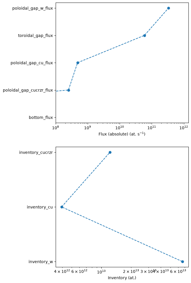
Post processing#
import matplotlib.pyplot as plt
import numpy as np
fig, axs = plt.subplots(nrows=2, ncols=1, figsize=(6, 12))
plt.sca(axs[0])
all_fluxes_vals = [np.abs(flux.data[0]) for flux in exports.values() if isinstance(flux, F.SurfaceFlux)]
all_fluxes_labels = [name for name, flux in exports.items() if isinstance(flux, F.SurfaceFlux)]
# sort
all_fluxes_vals, all_fluxes_labels = zip(*sorted(zip(all_fluxes_vals, all_fluxes_labels)))
plt.plot(all_fluxes_vals, all_fluxes_labels, marker="o", linestyle="--")
plt.xlabel("Flux (absolute) (at. s$^{-1}$)")
plt.xscale("log")
plt.xlim(left=1e8)
plt.sca(axs[1])
all_inventories_vals = [inv.data[0] for inv in exports.values() if isinstance(inv, F.TotalVolume)]
all_inventories_labels = [name for name, inv in exports.items() if isinstance(inv, F.TotalVolume)]
plt.plot(all_inventories_vals, all_inventories_labels, marker="o", linestyle="--")
plt.xlabel("Inventory (at.)")
plt.xscale("log")
plt.show()