Stepsize

Objectives:

• Set a stepsize for your simulation

• Accelerate your simulation with adaptive time stepping

• Ensure the simulation hits certain time milestones

Adaptive stepsize

It is often useful to have an adaptive stepsize that grows or shrink based on the difficulty of the solution.

FESTIM does that by allowing users to define their own F.Stepsize object.

The target_nb_iterations sets the optimal number of Newton iterations. If more iterations are required in order to converge, this might suggest that the problem is hard to solve and a smaller stepsize is required. On the other hand, when the solver converges very quickly, this may be possible to have larger stepsizes.

The parameter growth_factor defines by how much the stepsize is increased, and cutback_factor defines by how much it is shrunk.

Let’s demonstrate this with a simple example. Here we create an “empty” transient problem with no BCs, no source terms, nothing! The solution is \(c=0\) everywhere. We do this so that the number of iterations required to “converge” is always below target_nb_iterations, and the stepsize is increased everytime.

import festim as F
from dolfinx.mesh import create_unit_square
from mpi4py import MPI

fenics_mesh = create_unit_square(MPI.COMM_WORLD, 10, 10)
festim_mesh = F.Mesh(fenics_mesh)

my_model = F.HydrogenTransportProblem()

material_top = F.Material(D_0=1, E_D=0)

vol = F.VolumeSubdomain(id=1, material=material_top)

my_model.mesh = festim_mesh
my_model.subdomains = [vol]

H = F.Species("H")
my_model.species = [H]

my_model.settings = F.Settings(atol=1e-8, rtol=1e-8, final_time=1000)

my_model.temperature = 300

my_model.exports = [F.TotalVolume(field=H, volume=vol)]

/home/docs/checkouts/readthedocs.org/user_builds/festim-workshop/conda/latest/lib/python3.12/site-packages/festim/coupled_heat_hydrogen_problem.py:1: TqdmExperimentalWarning: Using `tqdm.autonotebook.tqdm` in notebook mode. Use `tqdm.tqdm` instead to force console mode (e.g. in jupyter console)
  import tqdm.autonotebook

We define a F.Stepsize object with an initial value of 10 and some typical control parameters:

my_model.settings.stepsize = F.Stepsize(
    initial_value=10,
    growth_factor=1.1,  # grow by 10%
    cutback_factor=0.9,  # shrink by 10%
    target_nb_iterations=4,  # target number of iterations per time step
)

Let’s run the adaptive time stepping model:

print("Running with adaptive time stepping...")
my_model.initialise()
my_model.run()
times_fast = my_model.exports[0].t

Running with adaptive time stepping...

Now, let’s replace the stepsize by a fixed stepsize and see how they compare:

print("Running with fixed time stepping...")
my_model.settings.stepsize = 10
my_model.initialise()
my_model.run()
times_slow = my_model.exports[0].t

Running with fixed time stepping...

Show code cell source

Hide code cell source

import matplotlib.pyplot as plt
import numpy as np

fig, axs = plt.subplots(2, 1, sharex=True)


def plot(times, label=None, annotate=True):
    steps = np.arange(len(times))
    dt = np.diff(times)

    axs[0].plot(steps[1:], dt, label=label)
    (l,) = axs[1].plot(steps, times, label=label)
    axs[1].scatter(steps[-1], times[-1], color=l.get_color())
    if annotate:
        axs[1].annotate(
            "Final time",
            (steps[-1], times[-1]),
            textcoords="offset points",
            xytext=(-10, -5),
            ha="right",
            color=l.get_color(),
        )


plot(times_fast, label="Adaptive time stepping")
plot(times_slow, label="Fixed time stepping")

axs[0].set_ylabel(r"Step size $\Delta t$")
axs[0].set_ylim(bottom=0)
axs[1].set_ylabel("Time $t$")
axs[0].legend(loc="upper right")
plt.xlabel("Timestep")

plt.show()

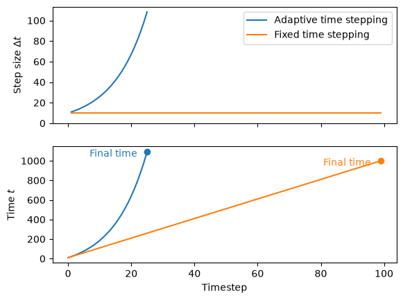
As expected, the stepsize is growing at each time step, meaning the final time is reached in just above 20 timesteps. Whereas for the fixed time stepping, it takes 100 iterations.

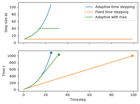
Stepsize can be capped by setting the parameter max_stepsize:

my_model.settings.stepsize = F.Stepsize(
    initial_value=10,
    growth_factor=1.1,  # grow by 10%
    cutback_factor=0.9,  # shrink by 10%
    target_nb_iterations=4,  # target number of iterations per time step
    max_stepsize=40, # maximum step size
)

my_model.initialise()
my_model.run()

capped_times = my_model.exports[0].t

Show code cell source

Hide code cell source

fig, axs = plt.subplots(2, 1, sharex=True)
plot(times_fast, label="Adaptive time stepping", annotate=False)
plot(times_slow, label="Fixed time stepping", annotate=False)
plot(capped_times, label="Adaptive with max", annotate=False)

axs[0].set_ylabel(r"Step size $\Delta t$")
axs[0].set_ylim(bottom=0)
axs[1].set_ylabel("Time $t$")
axs[0].legend(loc="upper right")
plt.xlabel("Timestep")

plt.show()

Milestones

Now that we know how to grow the stepsize to accelerate simulations, we have a new problem: what if we want the simulation to pass by a specific point in time but the timestep could be so big it completely misses it?

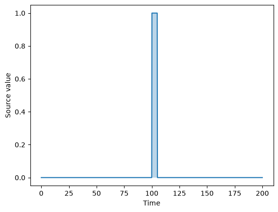
Let’s illustrate this by setting up a problem with a particle source only turning on only between 100 and 105 s, and \(c=0\) on the boundary.

import festim as F
from dolfinx.mesh import create_unit_square
from mpi4py import MPI

fenics_mesh = create_unit_square(MPI.COMM_WORLD, 10, 10)
festim_mesh = F.Mesh(fenics_mesh)

my_model = F.HydrogenTransportProblem()

material_top = F.Material(D_0=0.1, E_D=0)

vol = F.VolumeSubdomain(id=1, material=material_top)
boundary = F.SurfaceSubdomain(id=2, locator=lambda x: np.full_like(x[0], True))

my_model.mesh = festim_mesh
my_model.subdomains = [vol, boundary]

H = F.Species("H")
my_model.species = [H]

my_model.settings = F.Settings(atol=1e-8, rtol=1e-8, final_time=200)

my_model.temperature = 300

my_model.boundary_conditions = [
    F.FixedConcentrationBC(value=0, species=H, subdomain=boundary)
]

We set a time-dependent particle source term \(S\):

\[\begin{split} S = \begin{cases} 1, & \text{for } 100\leq t\leq 105\\ 0, & \text{otherwise } \end{cases} \end{split}\]

source_start = 100
source_end = 105

def source_value(t):
    if t <= source_end and t >= source_start:
        return 1
    else:
        return 0

my_model.sources = [
    F.ParticleSource(value=source_value, species=H, volume=vol)
]

Show code cell source

Hide code cell source

import matplotlib.pyplot as plt

times = np.linspace(0, 200, 1000)
source_values = [source_value(t) for t in times]
plt.plot(times, source_values)
plt.fill_between(times, source_values, alpha=0.3)

plt.xlabel("Time")
plt.ylabel("Source value")
plt.show()

We track the total quantity of H by adding a TotalVolume derived quantity:

my_model.exports = [F.TotalVolume(field=H, volume=vol)]

Then we set an adaptive timestep with a fairly large initial value:

my_model.settings.stepsize = F.Stepsize(
    initial_value=20,
    growth_factor=1.1,  # grow by 10%
    cutback_factor=0.9,  # shrink by 10%
    target_nb_iterations=4,  # target number of iterations per time step
)

my_model.initialise()
my_model.run()

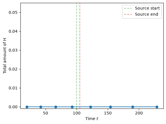
By plotting the values of TotalVolume we see that:

• the timesteps kind of jump over the time period of interest

• the value is zero all the time, which is WRONG!

Show code cell source

Hide code cell source

import matplotlib.pyplot as plt

plt.plot(my_model.exports[0].t, my_model.exports[0].data, marker="o")
plt.axvline(
    source_start, color="tab:green", alpha=0.5, linestyle="--", label="Source start"
)
plt.axvline(source_end, color="tab:red", alpha=0.5, linestyle="--", label="Source end")
plt.legend()
plt.xlabel("Time $t$")
plt.ylabel("Total amount of H")
plt.ylim(bottom=-0.001)
plt.show()

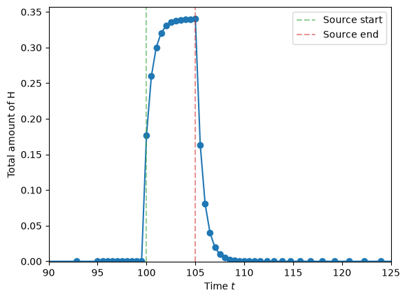
We can try and solve it first using milestones. Here we set a list of two milestones at the beginning and at the end of the source period:

my_model.settings.stepsize = F.Stepsize(
    initial_value=20,
    growth_factor=1.1,  # grow by 10%
    cutback_factor=0.9,  # shrink by 10%
    target_nb_iterations=4,  # target number of iterations per time step
    milestones=[source_start, source_end]
)

my_model.initialise()
my_model.run()

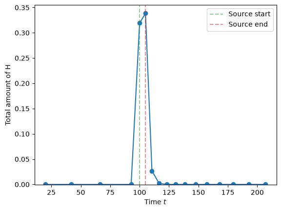
The result is already better, the solution is not zero all the time. But still, the solution looks a bit whacky… This is because, while the stepsize is modified (truncated) to hit the milestones, it is still fairly large during the time period of interest.

Show code cell source

Hide code cell source

plt.plot(my_model.exports[0].t, my_model.exports[0].data, marker="o")
plt.axvline(
    source_start, color="tab:green", alpha=0.5, linestyle="--", label="Source start"
)
plt.axvline(source_end, color="tab:red", alpha=0.5, linestyle="--", label="Source end")
plt.legend()
plt.xlabel("Time $t$")
plt.ylabel("Total amount of H")
plt.ylim(bottom=-0.001)
plt.show()

To improve it, let’s set the max_stepsize argument. Here we want the stepsize to be capped at 0.5 when the time is bewteen source_start - 5 and source_end + 5, otherwise, no limit (None).

We also modify the first milestone to hit just before the source is turned on.

We pass a lambda funtion to max_stepsize which is a function of t.

my_model.settings.stepsize = F.Stepsize(
    initial_value=20,
    growth_factor=1.1,  # grow by 10%
    cutback_factor=0.9,  # shrink by 10%
    target_nb_iterations=4,  # target number of iterations per time step
    milestones=[source_start - 5, source_end],
    max_stepsize=lambda t: 0.5 if source_start - 5 <= t <= source_end + 5 else None
)

my_model.initialise()
my_model.run()

Now the solution looks much smoother! 🎉

We can also see that the stepsize starts increasing again after ~115 s.

Show code cell source

Hide code cell source

plt.plot(my_model.exports[0].t, my_model.exports[0].data, marker="o")
plt.axvline(
    source_start, color="tab:green", alpha=0.5, linestyle="--", label="Source start"
)
plt.axvline(source_end, color="tab:red", alpha=0.5, linestyle="--", label="Source end")
plt.legend()
plt.xlabel("Time $t$")
plt.ylabel("Total amount of H")
plt.ylim(bottom=-0.001)
plt.xlim(source_start - 10, source_end + 20)
plt.show()