Hydrogen transport: examples#
This section discusses a few advanced examples using various boundary conditions to help users understand how BCs can help model their systems.
Objective:
Model plasma implantation using volumetric sources and approximations
Model complex multi-species isotopic exchange surface reactions
Modeling plasma implantation#
We can model plasma implantation using FESTIM’s ParticleSource class, which is a class used to define volumetric source terms. This is helpful in modeling thermo-desorption spectra (TDS) experiments or including the effect of plasma exposure on hydrogen transport.
Consider the following 1D plasma implantation problem, where we represent the plasma as a hydrogen source \(S_{ext}\) implanted on a tungsten material that is 20 microns thick:
where \(\varphi_{imp}\) is the implantation flux and \(f(x)\) is a Gaussian spatial distribution (distribution mean value represents implantation depth).
First, we setup a 1D mesh ranging from \( [0,L] \) and assign the subdomains and material properties for tungsten:
import festim as F
import ufl
import numpy as np

L = 20e-6
my_model = F.HydrogenTransportProblem()

vertices = np.concatenate(
    [
        np.linspace(0, 30e-9, num=200),
        np.linspace(3e-6, L, num=500),
    ]
)

my_model.mesh = F.Mesh1D(vertices)
Note
We break up the mesh region into two regions so we can refine the region closer to the implantation depth (defined below)
tungsten = F.Material(
    D_0=4.1e-07,  # m2/s
    E_D=0.39,  # eV
)
volume_subdomain = F.VolumeSubdomain1D(id=1, borders=[0, L], material=tungsten)
left_boundary = F.SurfaceSubdomain1D(id=1, x=0)
right_boundary = F.SurfaceSubdomain1D(id=2, x=L)

my_model.subdomains = [
    volume_subdomain,
    left_boundary,
    right_boundary,
]
Now, we define our incident_flux and gaussian_distribution function. Here, we define the mean implantation depth \(R_p\) and distribution width to be a few nanometers long:
incident_flux = 1e13
Rp = 4e-9
width = 2.5e-9

def gaussian_distribution(x, center, width):
    return (
        1
        / (width * (2 * ufl.pi) ** 0.5)
        * ufl.exp(-0.5 * ((x[0] - center) / width) ** 2)
    )
We can define our species and use ParticleSource to represent the source term, and then add it to our model:
H = F.Species("H")
my_model.species = [H]

source_term = F.ParticleSource(
    value=lambda x: incident_flux * gaussian_distribution(x, Rp, width),
    volume=volume_subdomain,
    species=H,
)

my_model.sources = [source_term]
Finally, we assign boundary conditions (zero concentration at \(x=0\) and \(x=L\)) and solve our problem:
my_model.boundary_conditions = [
    F.FixedConcentrationBC(subdomain=left_boundary, value=0, species=H),
    F.FixedConcentrationBC(subdomain=right_boundary, value=0, species=H),
]

my_model.temperature = 400
my_model.settings = F.Settings(atol=1e10, rtol=1e-10, transient=False)

profile_export = F.Profile1DExport(field=H,subdomain=volume_subdomain)
my_model.exports = [profile_export]

my_model.initialise()
my_model.run()
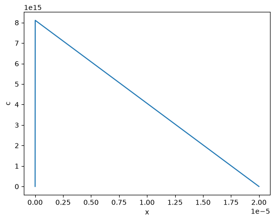
We see that a huge spike in concentration in the first few nanometers of tungesten, where the implantation range is focused.
Approximating plasma implantation using fixed concentration boundary conditions#
If recombination is fast enough, the spike shown above can be approximated as a fixed concentration boundary condition that mainly drives diffusion across the material. Learn more about the plasma implantation approximation approach here.
To see how we might approximate this, let’s define a maximum concentration to set on the left boundary, representing the spike from the implantation:
where \(\varphi_{imp}\) is the implantation flux and \(R_p\) is the implantation depth, both which we defined earlier, and \(D\) is the material diffusivity:
D = tungsten.D_0 * np.exp(-tungsten.E_D / (F.k_B * my_model.temperature))
c_m = incident_flux * Rp / D
Now, we’ll change our boundary conditions to represent the implantation as a fixed concentration on the left boundary, and remove the source term from our problem:
my_model.boundary_conditions = [
    F.FixedConcentrationBC(subdomain=left_boundary, value=c_m, species=H),
    F.FixedConcentrationBC(subdomain=right_boundary, value=0, species=H),
]

my_model.sources = []
profile_export = F.Profile1DExport(field=H,subdomain=volume_subdomain)
my_model.exports = [profile_export]

my_model.initialise()
my_model.run()
Let’s compare the profiles from the approximation to the volumetric source results:
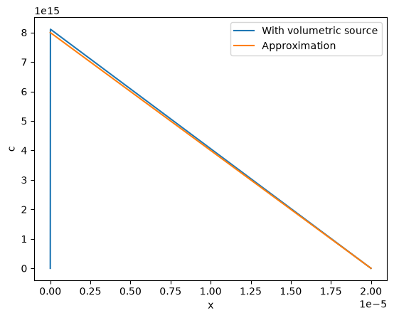
Using the approximation is computationally less expensive, and still provides similar diffusion profiles.
Complex isotopic exchange with multiple hydrogenic species#
Surface reactions can involve multiple hydrogen isotopes, allowing for the modeling of complex isotope-exchange mechanisms between species. For example, in a system with both mobile hydrogen and deuteriun, various molecular recombination pathways may occur at the surface, resulting in the formation of \(H_2\), \(D_2\), and \(HD\):
From this reaction scheme, the surface fluxes of H and D are:
Now consider the case where deuterium diffuses from left to right and reacts with background \(\mathrm{H_2}\), while \(\mathrm{P_{HD}}\) and \(\mathrm{P_{D_2}}\) are negligible at the surface. Formation of \(\mathrm{H}\) at the right boundary induces back-diffusion toward the left, even though none existed initially.
The boundary conditions for this scenario are:
First, let’s define a 1D mesh ranging from \(\mathrm{x=[0,1]}\):
import numpy as np
import festim as F

my_model = F.HydrogenTransportProblem()
my_model.mesh = F.Mesh1D(vertices=np.linspace(0, 1, 100))

left_surf = F.SurfaceSubdomain1D(id=1, x=0)
right_surf = F.SurfaceSubdomain1D(id=2, x=1)

material = F.Material(D_0=1e-2, E_D=0)
vol = F.VolumeSubdomain1D(id=1, borders=[0, 1], material=material)

my_model.subdomains = [vol, left_surf, right_surf]
Now, we define our species at recombination reactions using SurfaceReactionBC:
H = F.Species("H")
D = F.Species("D")
my_model.species = [H, D]

P_h2 = 1000

reaction_1_bc = F.SurfaceReactionBC(
    reactant=[H, D],
    gas_pressure=0,
    k_r0=1,
    E_kr=0.1,
    k_d0=1e-5,
    E_kd=0.1,
    subdomain=right_surf,
)

reaction_2_bc = F.SurfaceReactionBC(
    reactant=[D, D],
    gas_pressure=0,
    k_r0=1,
    E_kr=0.1,
    k_d0=1e-5,
    E_kd=0.1,
    subdomain=right_surf,
)

reaction_3_bc = F.SurfaceReactionBC(
    reactant=[H, H],
    gas_pressure=P_h2,
    k_r0=1,
    E_kr=0.1,
    k_d0=1e-5,
    E_kd=0.1,
    subdomain=right_surf,
)
Now, let’s add our isotopic exchange reaction using ParticleFluxBC (see here to learn more about defining isotopic exchange fluxes):
Kr_0_custom = 10000.0
E_Kr_custom = 0.5  # eV

def K_exchange(T):
    return Kr_0_custom * ufl.exp(-E_Kr_custom / (F.k_B * T))

def isotopic_exchange_D(c_D, T):
    return - K_exchange(T) * P_h2 * c_D

def isotopic_exchange_H(c_D, T):
    return + K_exchange(T) * P_h2 * c_D


reaction_4_D = F.ParticleFluxBC(
    value=isotopic_exchange_D,
    subdomain=right_surf,
    species_dependent_value={"c_D": D},
    species=D,
)

reaction_4_H = F.ParticleFluxBC(
    value=isotopic_exchange_H,
    subdomain=right_surf,
    species_dependent_value={"c_D": D},
    species=H,
)
Finally, we add our boundary conditions and solve the steady-state problem:
my_model.boundary_conditions = [
    reaction_1_bc,
    reaction_2_bc,
    reaction_3_bc,
    reaction_4_D,
    reaction_4_H,
    F.FixedConcentrationBC(subdomain=left_surf, value=1, species=D),
    F.FixedConcentrationBC(subdomain=left_surf, value=0, species=H),
]

my_model.temperature = 300

my_model.settings = F.Settings(atol=1e-10, rtol=1e-10, transient=False)

my_model.initialise()
my_model.run()
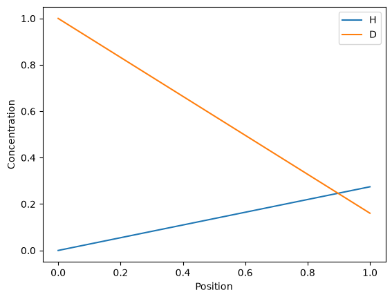
We see that the background \(\mathrm{H_2}\) reacts with the \(\mathrm{D}\), removing the total amount of \(\mathrm{D}\) from the surface. Conversely, the \(\mathrm{H}\) diffuses from the surface towards the left.