Derived quantities#
This tutorial goes over FESTIM’s built-in classes to help users export derived results.
Objectives:
Understanding how derived quantities are calculated
Exporting derived quantities in FESTIM
Working with data exported from FESTIM
Defining custom derived quantities
What is a derived quantity?#
This section summarizes how to compute common derived quantities in 1D/2D/3D FESTIM simulations. See the introduction section to learn more about when to export derived quantities.
Volume Quantities#
Volume quantities integrate or evaluate concentration over the computational domain \(\Omega\). For example, TotalVolume computes the total amount of hydrogen in the domain using the general expression:
where \(dV\) is the volume element. In 1D, \(dV = dx\) (length element); in 2D, \(dV = dA\) (area element); in 3D, \(dV = dV\) (volume element). This means the integral adapts to each dimension:
1D: \(\int_0^L c \, dx\) — integrating along a line
2D: \(\int_\Omega c \, dA\) — integrating over an area
3D: \(\int_\Omega c \, dV\) — integrating over a volume
The table below shows the dimension-specific expressions:
Derived Quantity |
1D Expression |
2D Expression |
3D Expression |
|---|---|---|---|
TotalVolume |
\(\int_0^L c \, dx\) [mol/m²] |
\(\int_\Omega c \, dA\) [mol/m] |
\(\int_\Omega c \, dV\) [mol] |
AverageVolume |
\(\frac{1}{L} \int_0^L c \, dx\) [mol/m³] |
\(\frac{1}{A} \int_\Omega c \, dA\) [mol/m³] |
\(\frac{1}{V} \int_\Omega c \, dV\) [mol/m³] |
MinimumVolume |
\(\min_{x \in [0,L]} c(x)\) [mol/m³] |
\(\min_{\mathbf{x} \in \Omega} c(\mathbf{x})\) [mol/m³] |
\(\min_{\mathbf{x} \in \Omega} c(\mathbf{x})\) [mol/m³] |
MaximumVolume |
\(\max_{x \in [0,L]} c(x)\) [mol/m³] |
\(\max_{\mathbf{x} \in \Omega} c(\mathbf{x})\) [mol/m³] |
\(\max_{\mathbf{x} \in \Omega} c(\mathbf{x})\) [mol/m³] |
Where: \(c\) is the concentration [mol/m³], \(L\) is the domain length, \(A\) is the domain area, \(V\) is the domain volume, \(\Omega\) is the domain, and \(\mathbf{x}\) is the position vector.
Warning
These integrals are in cartesian coordinates. See this open issue for non-cartesian derived quantities.
Surface Quantities#
Surface quantities integrate or evaluate concentration over a specific boundary surface \(\Gamma\). For example, TotalSurface computes the total amount of hydrogen on a given surface using the general expression:
where \(dS\) is the surface element and \(\Gamma\) is a specific boundary (e.g., the right surface in a 1D domain). In 1D, a “surface” is a single boundary point (0D); in 2D, \(dS = ds\) (arc length element); in 3D, \(dS = dS\) (area element). This means:
1D: \(c(x_0)\) — evaluating at a single boundary point (e.g., \(x_0 = 0\) or \(x_0 = L\))
2D: \(\int_\Gamma c \, ds\) — integrating along a boundary curve
3D: \(\int_\Gamma c \, dS\) — integrating over a boundary surface
The table below shows the dimension-specific expressions:
Derived Quantity |
1D Expression |
2D Expression |
3D Expression |
|---|---|---|---|
TotalSurface |
\(c(x_0)\) [mol/m³] |
\(\int_\Gamma c \, ds\) [mol/m²] |
\(\int_\Gamma c \, dS\) [mol/m] |
AverageSurface |
\(c(x_0)\) [mol/m³] |
\(\frac{1}{s} \int_\Gamma c \, ds\) [mol/m³] |
\(\frac{1}{S} \int_\Gamma c \, dS\) [mol/m³] |
MinimumSurface |
\(c(x_0)\) [mol/m³] |
\(\min_{\mathbf{x} \in \Gamma} c(\mathbf{x})\) [mol/m³] |
\(\min_{\mathbf{x} \in \Gamma} c(\mathbf{x})\) [mol/m³] |
MaximumSurface |
\(c(x_0)\) [mol/m³] |
\(\max_{\mathbf{x} \in \Gamma} c(\mathbf{x})\) [mol/m³] |
\(\max_{\mathbf{x} \in \Gamma} c(\mathbf{x})\) [mol/m³] |
SurfaceFlux |
\(-D \frac{dc}{dx}\bigg\rvert_{x_0}\) [mol/m²/s] |
\(\int_\Gamma-D \nabla c \cdot \mathbf{n}ds\) [mol/m/s] |
\(\int_\Gamma-D \nabla c \cdot \mathbf{n} dS\) [mol/s] |
Where: \(c\) is the concentration [mol/m³], \(D\) is the diffusion coefficient [m²/s], \(\mathbf{n}\) is the outward unit normal vector, \(\Gamma\) is a specific boundary surface, \(x_0\) is a boundary point (e.g., 0 or \(L\)), \(s\) is the arc length of the boundary curve (2D), \(S\) is the area of the boundary surface (3D), and \(\nabla c\) is the concentration gradient.
Warning
These integrals are in cartesian coordinates. See this open issue for non-cartesian derived quantities.
Note
The units for \(c\) are listed as \(\mathrm{mol/m^3}\) above, but there may be instances throughout this workshop where the concentration is listed in units of \(\mathrm{H/m^3}\), which refers to the number of hydrogen atoms per cubic meter. This is simply a unit conversion between \(n\), the number density of atoms, and molar concentration \(c_{mol}\) \(\mathrm{[mol/m^3]}\):
Exporting derived quantities in FESTIM#
Users can export derived values in FESTIM by passing in the desired field (which species to export), subdomain, and an optional filename (ending in .txt or .csv). For surface quantities, the subdomain should be a SurfaceSubdomain, while volume quantities should include a VolumeSubdomain input.
Let us consider a transient 2D diffusion problem with the following boundary conditions:
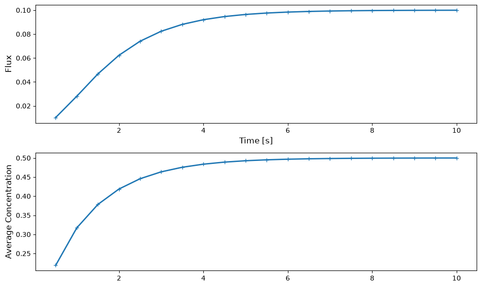
In this example, we will export derived values for the average volume concentration (over the entire region) and surface flux on the right surface for each timestep. Let us name the average volume and right flux quantities avg_vol and right_flux, respectively. By passing a value to the filename argument, it is possible to export the data to a csv file. Once the simulation is completed, we should see two files appear with those filenames:
avg_vol = F.AverageVolume(field=H, volume=vol, filename="avg_vol.csv")
right_flux = F.SurfaceFlux(field=H, surface=right_surface, filename="right_flux.csv")

my_model.exports = [
    avg_vol,
    right_flux
]

my_model.initialise()
my_model.run()
The export variables avg_vol and right_flux will have two attributes: data and t. The data attribute stores the values for the corresponding export, and t stores the timesteps of the simulation. For example, let us look at the avg_vol variable:
print(f"Average volume concentration: {avg_vol.data}")
print(f"Average volume timesteps: {avg_vol.t}")
Average volume concentration: [0.21905728666243415, 0.3169744491049101, 0.3783113983720679, 0.41870960237856947, 0.4456306467139692, 0.46362454631050815, 0.4756611487273429, 0.4837144726134959, 0.4891030161797746, 0.4927085899362626, 0.49512115590171074, 0.4967354568596908, 0.49781562147482505, 0.4985383836634673, 0.4990219999437085, 0.49934559837157344, 0.4995621252896525, 0.4997070082749765, 0.4998039527086059, 0.4998688203891775]
Average volume timesteps: [0.5, 1.0, 1.5, 2.0, 2.5, 3.0, 3.5, 4.0, 4.5, 5.0, 5.5, 6.0, 6.5, 7.0, 7.5, 8.0, 8.5, 9.0, 9.5, 10.0]
Post-processing of derived quantities#
Users can access derived quantities that have been exported from FESTIM by importing the .csv or .txt file.
Let us visualize the right_flux and avg_vol exports from the previous section. First, let’s import the files with numpy.loadtxt:
right_flux = np.loadtxt("right_flux.csv", delimiter=",", skiprows=1)
timesteps = right_flux[:, 0]
flux_values = right_flux[:, 1]

avg_vol = np.loadtxt("avg_vol.csv", delimiter=",", skiprows=1)
avg_vol_timesteps = avg_vol[:, 0]
avg_vol_values = avg_vol[:, 1]
Note
It would also be possible to directly use right_flux.data and right_flux.t instead of writing/reading a file.
Finally, we can plot both exports over time using matplotlib:
import matplotlib.pyplot as plt

fig, (ax1, ax2) = plt.subplots(figsize=(10, 6), nrows=2, ncols=1)

ax1.plot(timesteps, flux_values, linewidth=2, label='Right Surface Flux', marker="+")
ax1.set_xlabel('Time [s]', fontsize=12)
ax1.set_ylabel('Flux', fontsize=12)

ax2.plot(avg_vol_timesteps, avg_vol_values, linewidth=2, label='Average Volume Concentration', marker="+")
ax2.set_ylabel('Average Concentration', fontsize=12)

plt.tight_layout()
plt.show()
Custom derived quantities#
Added in version 2.0: CustomQuantity was introduced in FESTIM 2.0.
The built-in quantities above cover the most common needs, but sometimes you want to integrate an arbitrary expression over a volume or a surface. This is what CustomQuantity is for: you provide a callable that returns a UFL expression, and FESTIM integrates it over the chosen subdomain:
The callable receives keyword arguments assembled by the problem. The most useful entries are:
Keyword |
Meaning |
|---|---|
species name (e.g. |
the concentration of that species |
|
the temperature field |
|
the diffusion coefficient (overall, or per species) |
|
the outward facet normal (for surface subdomains) |
|
the spatial coordinate |
Let us reuse a steady-state 2D problem with \(c_H = 1\) on the left and \(c_H = 0\) on the right:
We define two custom quantities. The first integrates \(c_H^2\) over the volume; the second computes the diffusion flux \(-D\,\nabla c_H \cdot \mathbf{n}\) on the right surface (which reproduces the built-in SurfaceFlux). Note the use of ufl to build the expression:
import ufl

volume_quantity = F.CustomQuantity(
    expr=lambda **kwargs: kwargs["H"] ** 2,
    subdomain=vol,
    title="int of c^2",
)

surface_quantity = F.CustomQuantity(
    expr=lambda **kwargs: -kwargs["D"] * ufl.dot(ufl.grad(kwargs["H"]), kwargs["n"]),
    subdomain=right_surface,
    title="custom flux",
)

my_model.exports = [volume_quantity, surface_quantity]
my_model.initialise()
my_model.run()
Just like the built-in quantities, the results are stored in the data and t attributes:
print(f"Volume integral of c^2: {volume_quantity.data}")
print(f"Custom surface flux: {surface_quantity.data}")
Volume integral of c^2: [0.33333333333333287]
Custom surface flux: [0.09999999999999969]
Tip
Because expr can be any UFL expression, CustomQuantity is a convenient way to export quantities that don’t have a dedicated class, such as a recombination flux \(q = K_r\, c^2\) on a surface, or a temperature-weighted average in the volume.