Simple simulation

In this task, we’ll go through the basics of FESTIM and run a simple simulation on a 1D domain.

The very first step is to import the festim package:

import festim as F

print(F.__version__)

/home/docs/checkouts/readthedocs.org/user_builds/festim-workshop/conda/latest/lib/python3.12/site-packages/festim/coupled_heat_hydrogen_problem.py:1: TqdmExperimentalWarning: Using `tqdm.autonotebook.tqdm` in notebook mode. Use `tqdm.tqdm` instead to force console mode (e.g. in jupyter console)
  import tqdm.autonotebook

2.0b2.post2

We then create a HydrogenTransportProblem object.

my_model = F.HydrogenTransportProblem()

Mesh

FESTIM simulations need a mesh, here we use Mesh1D.

import numpy as np

my_model.mesh = F.Mesh1D(vertices=np.linspace(0, 1, num=1001))

See also

For more information on meshes in FESTIM, see Meshes.

Materials

Material objects hold the materials properties like diffusivity.

mat = F.Material(D_0=1, E_D=0.0)

volume_subdomain = F.VolumeSubdomain1D(id=1, borders=[0, 1], material=mat)
boundary_left = F.SurfaceSubdomain1D(id=1, x=0)
boundary_right = F.SurfaceSubdomain1D(id=2, x=1)
my_model.subdomains = [volume_subdomain, boundary_left, boundary_right]

H = F.Species("H")
my_model.species = [H]

Temperature

my_model.temperature = 300

Boundary conditions

Our hydrogen transport problem now needs boundary conditions.

my_model.boundary_conditions = [
    F.FixedConcentrationBC(subdomain=boundary_left, value=1, species=H),
    F.FixedConcentrationBC(subdomain=boundary_right, value=0, species=H),
]

Settings

With Settings we set the main solver parameters.

my_model.settings = F.Settings(atol=1e-10, rtol=1e-10, final_time=2)

Stepsize

Since we are solving a transient problem, we need to set a Stepsize. Here, the value of the stepsize is fixed at 0.05.

my_model.settings.stepsize = F.Stepsize(0.05, milestones=[0.05, 0.1, 0.2, 0.5, 1])  # s

Exports

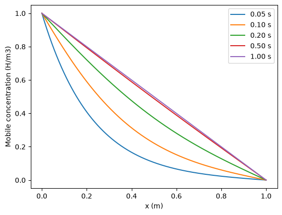
Finally, we want to be able to visualise the concentration field.

profile = F.Profile1DExport(field=H, subdomain=volume_subdomain, times=my_model.settings.stepsize.milestones)

my_model.exports = [
    F.VTXSpeciesExport(
        field=H,
        filename="hydrogen_concentration.bp",
    ),
    profile,
]

Run

Finally, we initialise the model and run it!

my_model.initialise()

my_model.run()

You should now see the file hydrogen_concentration.bp.

See also

Check out the Paraview section for visualisation!

Visualise

import matplotlib.pyplot as plt

x = my_model.mesh.mesh.geometry.x[:, 0]
for time, data in zip(profile.t, profile.data):
    plt.plot(x, data, label=f"{time} s")

plt.xlabel("x (m)")
plt.ylabel("Mobile concentration (H/m3)")
plt.legend()
plt.show()